DBSCAN

Machine learning and data mining
Problems Classification Clustering Regression Anomaly detection Association rules Reinforcement learning Structured prediction Feature engineering Feature learning Online learning Semi-supervised learning Unsupervised learning Learning to rank Grammar induction
Supervised learning (classification • regression) Decision trees Ensembles (Bagging, Boosting, Random forest) k-NN Linear regression Naive Bayes Neural networks Logistic regression Perceptron Relevance vector machine (RVM) Support vector machine (SVM)
Clustering BIRCH Hierarchical k-means Expectation-maximization (EM) DBSCAN OPTICS Mean-shift
Dimensionality reduction Factor analysis CCA ICA LDA NMF PCA t-SNE
Structured prediction Graphical models (Bayes net, CRF, HMM)
Anomaly detection k-NN Local outlier factor
Neural nets Autoencoder Deep learning Multilayer perceptron RNN Restricted Boltzmann machine SOM Convolutional neural network
Reinforcement Learning Q-Learning SARSA Temporal Difference (TD)
Theory Bias-variance dilemma Computational learning theory Empirical risk minimization Occam learning PAC learning Statistical learning VC theory
Machine learning venues NIPS ICML IJMLC ML JMLR ArXiv:cs.LG
Machine learning portal

Density-based spatial clustering of applications with noise (DBSCAN) is a data clustering algorithm proposed by Martin Ester, Hans-Peter Kriegel, Jörg Sander and Xiaowei Xu in 1996.^[1] It is a density-based clustering algorithm: given a set of points in some space, it groups together points that are closely packed together (points with many nearby neighbors), marking as outliers points that lie alone in low-density regions (whose nearest neighbors are too far away). DBSCAN is one of the most common clustering algorithms and also most cited in scientific literature.^[2]

In 2014, the algorithm was awarded the test of time award (an award given to algorithms which have received substantial attention in theory and practice) at the leading data mining conference, KDD.^[3]

Preliminary

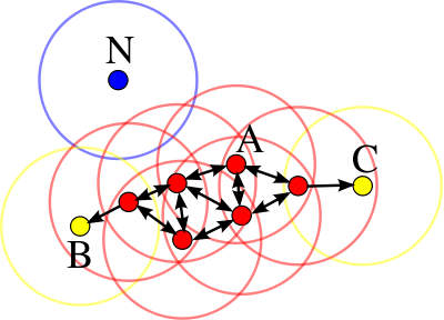
Consider a set of points in some space to be clustered. For the purpose of DBSCAN clustering, the points are classified as core points, (density-)reachable points and outliers, as follows:

• A point p is a core point if at least minPts points are within distance ε(ε is the maximum radius of the neighborhood from p) of it (including p). Those points are said to be directly reachable from p. By definition, no points are directly reachable from a non-core point.
• A point q is reachable from p if there is a path p₁, ..., p_n with p₁ = p and p_n = q, where each p_i+1 is directly reachable from p_i (all the points on the path must be core points, with the possible exception of q).
• All points not reachable from any other point are outliers.

Now if p is a core point, then it forms a cluster together with all points (core or non-core) that are reachable from it. Each cluster contains at least one core point; non-core points can be part of a cluster, but they form its "edge", since they cannot be used to reach more points.

In this diagram, minPts = 4. Point A and the other red points are core points, because the area surrounding these points in an ε radius contain at least 4 points (including the point itself). Because they are all reachable from one another, they form a single cluster. Points B and C are not core points, but are reachable from A (via other core points) and thus belong to the cluster as well. Point N is a noise point that is neither a core point nor density-reachable.

Reachability is not a symmetric relation since, by definition, no point may be reachable from a non-core point, regardless of distance (so a non-core point may be reachable, but nothing can be reached from it). Therefore a further notion of connectedness is needed to formally define the extent of the clusters found by DBSCAN. Two points p and q are density-connected if there is a point o such that both p and q are density-reachable from o. Density-connectedness is symmetric.

A cluster then satisfies two properties:

1. All points within the cluster are mutually density-connected.
2. If a point is density-reachable from any point of the cluster, it is part of the cluster as well.

Algorithm

DBSCAN requires two parameters: ε (eps) and the minimum number of points required to form a dense region^{[lower-alpha 1]} (minPts). It starts with an arbitrary starting point that has not been visited. This point's ε-neighborhood is retrieved, and if it contains sufficiently many points, a cluster is started. Otherwise, the point is labeled as noise. Note that this point might later be found in a sufficiently sized ε-environment of a different point and hence be made part of a cluster.

If a point is found to be a dense part of a cluster, its ε-neighborhood is also part of that cluster. Hence, all points that are found within the ε-neighborhood are added, as is their own ε-neighborhood when they are also dense. This process continues until the density-connected cluster is completely found. Then, a new unvisited point is retrieved and processed, leading to the discovery of a further cluster or noise.

The algorithm can be expressed as follows, in pseudocode following the original published nomenclature:^[1]

DBSCAN(D, eps, MinPts) {
   C = 0
   for each point P in dataset D {
      if P is visited
         continue next point
      mark P as visited
      NeighborPts = regionQuery(P, eps)
      if sizeof(NeighborPts) < MinPts
         mark P as NOISE
      else {
         C = next cluster
         expandCluster(P, NeighborPts, C, eps, MinPts)
      }
   }
}

expandCluster(P, NeighborPts, C, eps, MinPts) {
   add P to cluster C
   for each point P' in NeighborPts { 
      if P' is not visited {
         mark P' as visited
         NeighborPts' = regionQuery(P', eps)
         if sizeof(NeighborPts') >= MinPts
            NeighborPts = NeighborPts joined with NeighborPts'
      }
      if P' is not yet member of any cluster
         add P' to cluster C
   }
}

regionQuery(P, eps)
   return all points within P's eps-neighborhood (including P)

Note that the algorithm can be simplified by merging the per-point "has been visited" and "belongs to cluster C" logic, as well as by inlining the contents of the "expandCluster" subroutine, which is only called from one place. These simplifications have been omitted from the above pseudocode in order to reflect the originally published version. Additionally, the regionQuery function need not return P in the list of points to be visited, as long as it is otherwise still counted in the local density estimate.

Complexity

DBSCAN visits each point of the database, possibly multiple times (e.g., as candidates to different clusters). For practical considerations, however, the time complexity is mostly governed by the number of regionQuery invocations. DBSCAN executes exactly one such query for each point, and if an indexing structure is used that executes a neighborhood query in O(log n), an overall average runtime complexity of O(n log n) is obtained (if parameter ε is chosen in a meaningful way, i.e. such that on average only O(log n) points are returned). Without the use of an accelerating index structure, or on degenerated data (e.g. all points within a distance less than ε), the worst case run time complexity remains O(n²). The distance matrix of size (n²-n)/2 can be materialized to avoid distance recomputations, but this needs O(n²) memory, whereas a non-matrix based implementation of DBSCAN only needs O(n) memory.

DBSCAN can find non-linearly separable clusters. This dataset cannot be adequately clustered with k-means or Gaussian Mixture EM clustering.

Advantages

1. DBSCAN does not require one to specify the number of clusters in the data a priori, as opposed to k-means.
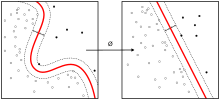
2. DBSCAN can find arbitrarily shaped clusters. It can even find a cluster completely surrounded by (but not connected to) a different cluster. Due to the MinPts parameter, the so-called single-link effect (different clusters being connected by a thin line of points) is reduced.
3. DBSCAN has a notion of noise, and is robust to outliers.
4. DBSCAN requires just two parameters and is mostly insensitive to the ordering of the points in the database. (However, points sitting on the edge of two different clusters might swap cluster membership if the ordering of the points is changed, and the cluster assignment is unique only up to isomorphism.)
5. DBSCAN is designed for use with databases that can accelerate region queries, e.g. using an R* tree.
6. The parameters minPts and ε can be set by a domain expert, if the data is well understood.

Disadvantages

1. DBSCAN is not entirely deterministic: border points that are reachable from more than one cluster can be part of either cluster, depending on the order the data is processed. Fortunately, this situation does not arise often, and has little impact on the clustering result: both on core points and noise points, DBSCAN is deterministic. DBSCAN*^[4] is a variation that treats border points as noise, and this way achieves a fully deterministic result as well as a more consistent statistical interpretation of density-connected components.
2. The quality of DBSCAN depends on the distance measure used in the function regionQuery(P,ε). The most common distance metric used is Euclidean distance. Especially for high-dimensional data, this metric can be rendered almost useless due to the so-called "Curse of dimensionality", making it difficult to find an appropriate value for ε. This effect, however, is also present in any other algorithm based on Euclidean distance.
3. DBSCAN cannot cluster data sets well with large differences in densities, since the minPts-ε combination cannot then be chosen appropriately for all clusters.
4. If the data and scale are not well understood, choosing a meaningful distance threshold ε can be difficult.

See the section below on extensions for algorithmic modifications to handle these issues.

Parameter estimation

Every data mining task has the problem of parameters. Every parameter influences the algorithm in specific ways. For DBSCAN, the parameters ε and minPts are needed. The parameters must be specified by the user. Ideally, the value of ε is given by the problem to solve (e.g. a physical distance), and minPts is then the desired minimum cluster size.^{[lower-alpha 1]}

• MinPts: As a rule of thumb, a minimum minPts can be derived from the number of dimensions D in the data set, as minPts ≥ D + 1. The low value of minPts = 1 does not make sense, as then every point on its own will already be a cluster. With minPts ≤ 2, the result will be the same as of hierarchical clustering with the single link metric, with the dendrogram cut at height ε. Therefore, minPts must be chosen at least 3. However, larger values are usually better for data sets with noise and will yield more significant clusters. The larger the data set, the larger the value of minPts should be chosen.
• ε: The value for ε can then be chosen by using a k-distance graph, plotting the distance to the k = minPts nearest neighbor. Good values of ε are where this plot shows a strong bend: if ε is chosen much too small, a large part of the data will not be clustered; whereas for a too high value of ε, clusters will merge and the majority of objects will be in the same cluster. In general, small values of ε are preferable, and as a rule of thumb only a small fraction of points should be within this distance of each other.
• Distance function: The choice of distance function is tightly coupled to the choice of ε, and has a major impact on the results. In general, it will be necessary to first identify a reasonable measure of similarity for the data set, before the parameter ε can be chosen.

OPTICS can be seen as a generalization of DBSCAN that replaces the ε parameter with a maximum value that mostly affects performance. MinPts then essentially becomes the minimum cluster size to find. While the algorithm is much easier to parameterize than DBSCAN, the results are a bit more difficult to use, as it will usually produce a hierarchical clustering instead of the simple data partitioning that DBSCAN produces.

Recently, one of the original authors of DBSCAN has revisited DBSCAN and OPTICS, and published a refined version of hierarchical DBSCAN (HDBSCAN*),^[4][5] which no longer has the notion of border points.

Extensions

Generalized DBSCAN (GDBSCAN)^[6][7] is a generalization by the same authors to arbitrary "neighborhood" and "dense" predicates. The ε and minpts parameters are removed from the original algorithm and moved to the predicates. For example, on polygon data, the "neighborhood" could be any intersecting polygon, whereas the density predicate uses the polygon areas instead of just the object count.

Various extensions to the DBSCAN algorithm have been proposed, including methods for parallelization, parameter estimation, and support for uncertain data. The basic idea has been extended to hierarchical clustering by the OPTICS algorithm. DBSCAN is also used as part of subspace clustering algorithms like PreDeCon and SUBCLU. HDBSCAN^[4] is a hierarchical version of DBSCAN which is also faster than OPTICS, from which a flat partition consisting of the most prominent clusters can be extracted from the hierarchy.^[5]

Availability

Different implementations of the same algorithm were found to exhibit enormous performance differences, with the fastest on a test data set finishing in 1.4 seconds, the slowest taking 13803 seconds.^[8] The differences can be attributed to implementation quality, language and compiler differences, and the use of indexes for acceleration.

• Apache Commons Math contains a Java implementation of the algorithm running in quadratic time.
• ELKI offers an implementation of DBSCAN as well as GDBSCAN and other variants. This implementation can use various index structures for sub-quadratic runtime and supports arbitrary distance functions and arbitrary data types, but it may be outperformed by low-level optimized (and specialized) implementations on small data sets.
• R contains DBSCAN in the fpc package with support for arbitrary distance functions via distance matrices. However it does not have index support (and thus has quadratic runtime and memory complexity) and is rather slow due to the R interpreter. A faster version is implemented in C++ using kd-trees (for Euclidean distance only) in the R package dbscan.
• scikit-learn includes a Python implementation of DBSCAN for arbitrary Minkowski metrics, which can be accelerated using kd-trees and ball trees but which uses worst-case quadratic memory.
• SPMF offers a GPL-V3 Java implementation of the DBSCAN algorithm with KD-Tree support (for Euclidean distance only).
• Weka contains (as an optional package in latest versions) a basic implementation of DBSCAN that runs in quadratic time and linear memory.

See also

• OPTICS algorithm: a generalization of DBSCAN to multiple ranges, effectively replacing the ε parameter with a maximum search radius.
• Connected component
• Disjoint-set data structure

Notes

References

Further reading

• Arlia, Domenica; Coppola, Massimo. "Experiments in Parallel Clustering with DBSCAN". Euro-Par 2001: Parallel Processing: 7th International Euro-Par Conference Manchester, UK August 28–31, 2001, Proceedings. Springer Berlin. 
• Kriegel, Hans-Peter; Kröger, Peer; Sander, Jörg; Zimek, Arthur (2011). "Density-based Clustering". WIREs Data Mining and Knowledge Discovery. 1 (3): 231–240. doi:10.1002/widm.30.

References

- 1 2 Ester, Martin; Kriegel, Hans-Peter; Sander, Jörg; Xu, Xiaowei (1996). Simoudis, Evangelos; Han, Jiawei; Fayyad, Usama M., eds. A density-based algorithm for discovering clusters in large spatial databases with noise. Proceedings of the Second International Conference on Knowledge Discovery and Data Mining (KDD-96). AAAI Press. pp. 226–231. CiteSeerX 10.1.1.121.9220
. ISBN 1-57735-004-9.
- ↑ Most cited data mining articles according to Microsoft academic search; DBSCAN is on rank 24, when accessed on: 4/18/2010
- ↑ "2014 SIGKDD Test of Time Award". ACM SIGKDD. 2014-08-18. Retrieved 2016-07-27.
- 1 2 3 Campello, R. J. G. B.; Moulavi, D.; Sander, J. (2013). Density-Based Clustering Based on Hierarchical Density Estimates. Proceedings of the 17th Pacific-Asia Conference on Knowledge Discovery in Databases, PAKDD 2013. Lecture Notes in Computer Science. 7819. p. 160. doi:10.1007/978-3-642-37456-2_14. ISBN 978-3-642-37455-5.
- 1 2 Campello, R. J. G. B.; Moulavi, D.; Zimek, A.; Sander, J. (2013). "A framework for semi-supervised and unsupervised optimal extraction of clusters from hierarchies". Data Mining and Knowledge Discovery. 27 (3): 344. doi:10.1007/s10618-013-0311-4.
- ↑ Sander, Jörg; Ester, Martin; Kriegel, Hans-Peter; Xu, Xiaowei (1998). "Density-Based Clustering in Spatial Databases: The Algorithm GDBSCAN and Its Applications". Data Mining and Knowledge Discovery. Berlin: Springer-Verlag. 2 (2): 169–194. doi:10.1023/A:1009745219419.
- ↑ Sander, Jörg (1998). Generalized Density-Based Clustering for Spatial Data Mining. München: Herbert Utz Verlag. ISBN 3-89675-469-6.
- ↑ Kriegel, Hans-Peter; Schubert, Erich; Zimek, Arthur (2016). "The (black) art of runtime evaluation: Are we comparing algorithms or implementations?". Knowledge and Information Systems. doi:10.1007/s10115-016-1004-2. ISSN 0219-1377.