k-d tree
| k-d tree | ||
|---|---|---|
| Type | Multidimensional BST | |
| Invented | 1975 | |
| Invented by | Jon Louis Bentley | |
| Time complexity in big O notation | ||
| Average | Worst case | |
| Space | O(n) | O(n) |
| Search | O(log n) | O(n) |
| Insert | O(log n) | O(n) |
| Delete | O(log n) | O(n) |

In computer science, a k-d tree (short for k-dimensional tree) is a space-partitioning data structure for organizing points in a k-dimensional space. k-d trees are a useful data structure for several applications, such as searches involving a multidimensional search key (e.g. range searches and nearest neighbor searches). k-d trees are a special case of binary space partitioning trees.
Informal description
The k-d tree is a binary tree in which every node is a k-dimensional point. Every non-leaf node can be thought of as implicitly generating a splitting hyperplane that divides the space into two parts, known as half-spaces. Points to the left of this hyperplane are represented by the left subtree of that node and points right of the hyperplane are represented by the right subtree. The hyperplane direction is chosen in the following way: every node in the tree is associated with one of the k-dimensions, with the hyperplane perpendicular to that dimension's axis. So, for example, if for a particular split the "x" axis is chosen, all points in the subtree with a smaller "x" value than the node will appear in the left subtree and all points with larger "x" value will be in the right subtree. In such a case, the hyperplane would be set by the x-value of the point, and its normal would be the unit x-axis.[1]
Operations on k-d trees
Construction
Since there are many possible ways to choose axis-aligned splitting planes, there are many different ways to construct k-d trees. The canonical method of k-d tree construction has the following constraints:[2]
- As one moves down the tree, one cycles through the axes used to select the splitting planes. (For example, in a 3-dimensional tree, the root would have an x-aligned plane, the root's children would both have y-aligned planes, the root's grandchildren would all have z-aligned planes, the root's great-grandchildren would all have x-aligned planes, the root's great-great-grandchildren would all have y-aligned planes, and so on.)
- Points are inserted by selecting the median of the points being put into the subtree, with respect to their coordinates in the axis being used to create the splitting plane. (Note the assumption that we feed the entire set of n points into the algorithm up-front.)
This method leads to a balanced k-d tree, in which each leaf node is approximately the same distance from the root. However, balanced trees are not necessarily optimal for all applications.
Note that it is not required to select the median point. In the case where median points are not selected, there is no guarantee that the tree will be balanced. To avoid coding a complex O(n) median-finding algorithm[3][4] or using an O(n log n) sort such as Heapsort or Mergesort to sort all n points, a popular practice is to sort a fixed number of randomly selected points, and use the median of those points to serve as the splitting plane. In practice, this technique often results in nicely balanced trees.
Given a list of n points, the following algorithm uses a median-finding sort to construct a balanced k-d tree containing those points.
function kdtree (list of points pointList, int depth)
{
    // Select axis based on depth so that axis cycles through all valid values
    var int axis := depth mod k;

    // Sort point list and choose median as pivot element
    select median by axis from pointList;

    // Create node and construct subtrees
    var tree_node node;
    node.location := median;
    node.leftChild := kdtree(points in pointList before median, depth+1);
    node.rightChild := kdtree(points in pointList after median, depth+1);
    return node;
}
It is common that points "after" the median include only the ones that are strictly greater than the median. For points that lie on the median, it is possible to define a "superkey" function that compares the points in all dimensions. In some cases, it is acceptable to let points equal to the median lie on one side of the median, for example, by splitting the points into a "lesser than" subset and a "greater than or equal to" subset.
|
The above algorithm implemented in the Python programming language is as follows: from collections import namedtuple
from operator import itemgetter
from pprint import pformat
class Node(namedtuple('Node', 'location left_child right_child')):
def __repr__(self):
return pformat(tuple(self))
def kdtree(point_list, depth=0):
try:
k = len(point_list[0]) # assumes all points have the same dimension
except IndexError as e: # if not point_list:
return None
# Select axis based on depth so that axis cycles through all valid values
axis = depth % k
# Sort point list and choose median as pivot element
point_list.sort(key=itemgetter(axis))
median = len(point_list) // 2 # choose median
# Create node and construct subtrees
return Node(
location=point_list[median],
left_child=kdtree(point_list[:median], depth + 1),
right_child=kdtree(point_list[median + 1:], depth + 1)
)
def main():
"""Example usage"""
point_list = [(2,3), (5,4), (9,6), (4,7), (8,1), (7,2)]
tree = kdtree(point_list)
print(tree)
if __name__ == '__main__':
main()
Output would be: ((7, 2),
((5, 4), ((2, 3), None, None), ((4, 7), None, None)),
((9, 6), ((8, 1), None, None), None))
The generated tree is shown below. 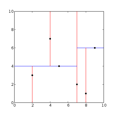 k-d tree decomposition for the point set (2,3), (5,4), (9,6), (4,7), (8,1), (7,2). The resulting k-d tree. |
This algorithm creates the invariant that for any node, all the nodes in the left subtree are on one side of a splitting plane, and all the nodes in the right subtree are on the other side. Points that lie on the splitting plane may appear on either side. The splitting plane of a node goes through the point associated with that node (referred to in the code as node.location).
Alternative algorithms for building a balanced k-d tree presort the data prior to building the tree. Then, they maintain the order of the presort during tree construction and hence eliminate the costly step of finding the median at each level of subdivision. Two such algorithms build a balanced k-d tree to sort triangles in order to improve the execution time of ray tracing for three-dimensional computer graphics. These algorithms presort n triangles prior to building the k-d tree, then build the tree in O(n log n) time in the best case.[5][6] An algorithm that builds a balanced k-d tree to sort points has a worst-case complexity of O(kn log n).[7] This algorithm presorts n points in each of k dimensions using an O(n log n) sort such as Heapsort or Mergesort prior to building the tree. It then maintains the order of these k presorts during tree construction and thereby avoids finding the median at each level of subdivision.
Adding elements
One adds a new point to a k-d tree in the same way as one adds an element to any other search tree. First, traverse the tree, starting from the root and moving to either the left or the right child depending on whether the point to be inserted is on the "left" or "right" side of the splitting plane. Once you get to the node under which the child should be located, add the new point as either the left or right child of the leaf node, again depending on which side of the node's splitting plane contains the new node.
Adding points in this manner can cause the tree to become unbalanced, leading to decreased tree performance. The rate of tree performance degradation is dependent upon the spatial distribution of tree points being added, and the number of points added in relation to the tree size. If a tree becomes too unbalanced, it may need to be re-balanced to restore the performance of queries that rely on the tree balancing, such as nearest neighbour searching.
Removing elements
To remove a point from an existing k-d tree, without breaking the invariant, the easiest way is to form the set of all nodes and leaves from the children of the target node, and recreate that part of the tree.
Another approach is to find a replacement for the point removed.[8] First, find the node R that contains the point to be removed. For the base case where R is a leaf node, no replacement is required. For the general case, find a replacement point, say p, from the subtree rooted at R. Replace the point stored at R with p. Then, recursively remove p.
For finding a replacement point, if R discriminates on x (say) and R has a right child, find the point with the minimum x value from the subtree rooted at the right child. Otherwise, find the point with the maximum x value from the subtree rooted at the left child.
Balancing
Balancing a k-d tree requires care because k-d trees are sorted in multiple dimensions so the tree rotation technique cannot be used to balance them as this may break the invariant.
Several variants of balanced k-d trees exist. They include divided k-d tree, pseudo k-d tree, k-d B-tree, hB-tree and Bkd-tree. Many of these variants are adaptive k-d trees.
Nearest neighbour search

The nearest neighbour search (NN) algorithm aims to find the point in the tree that is nearest to a given input point. This search can be done efficiently by using the tree properties to quickly eliminate large portions of the search space.
Searching for a nearest neighbour in a k-d tree proceeds as follows:
- Starting with the root node, the algorithm moves down the tree recursively, in the same way that it would if the search point were being inserted (i.e. it goes left or right depending on whether the point is lesser than or greater than the current node in the split dimension).
- Once the algorithm reaches a leaf node, it saves that node point as the "current best"
- The algorithm unwinds the recursion of the tree, performing the following steps at each node:
- If the current node is closer than the current best, then it becomes the current best.
- The algorithm checks whether there could be any points on the other side of the splitting plane that are closer to the search point than the current best. In concept, this is done by intersecting the splitting hyperplane with a hypersphere around the search point that has a radius equal to the current nearest distance. Since the hyperplanes are all axis-aligned this is implemented as a simple comparison to see whether the distance between the splitting coordinate of the search point and current node is lesser than the distance (overall coordinates) from the search point to the current best.
- If the hypersphere crosses the plane, there could be nearer points on the other side of the plane, so the algorithm must move down the other branch of the tree from the current node looking for closer points, following the same recursive process as the entire search.
- If the hypersphere doesn't intersect the splitting plane, then the algorithm continues walking up the tree, and the entire branch on the other side of that node is eliminated.
- When the algorithm finishes this process for the root node, then the search is complete.
Generally the algorithm uses squared distances for comparison to avoid computing square roots. Additionally, it can save computation by holding the squared current best distance in a variable for comparison.
Finding the nearest point is an O(log n) operation in the case of randomly distributed points, although analysis in general is tricky. However an algorithm has been given that claims guaranteed O(log n) complexity.[9]
In high-dimensional spaces, the curse of dimensionality causes the algorithm to need to visit many more branches than in lower-dimensional spaces. In particular, when the number of points is only slightly higher than the number of dimensions, the algorithm is only slightly better than a linear search of all of the points.
The algorithm can be extended in several ways by simple modifications. It can provide the k nearest neighbours to a point by maintaining k current bests instead of just one. A branch is only eliminated when k points have been found and the branch cannot have points closer than any of the k current bests.
It can also be converted to an approximation algorithm to run faster. For example, approximate nearest neighbour searching can be achieved by simply setting an upper bound on the number points to examine in the tree, or by interrupting the search process based upon a real time clock (which may be more appropriate in hardware implementations). Nearest neighbour for points that are in the tree already can be achieved by not updating the refinement for nodes that give zero distance as the result, this has the downside of discarding points that are not unique, but are co-located with the original search point.
Approximate nearest neighbour is useful in real-time applications such as robotics due to the significant speed increase gained by not searching for the best point exhaustively. One of its implementations is best-bin-first search.
Range search
A range search searches for ranges of parameters. For example, if a tree is storing values corresponding to income and age, then a range search might be something like looking for all members of the tree which have an age between 20 and 50 years and an income between 50,000 and 80,000. Since k-d trees divide the range of a domain in half at each level of the tree, they are useful for performing range searches.
Analyses of binary search trees has found that the worst case time for range search in a k-dimensional KD tree containing N nodes is given by the following equation.[10]

High-dimensional data
k-d trees are not suitable for efficiently finding the nearest neighbour in high-dimensional spaces. As a general rule, if the dimensionality is k, the number of points in the data, N, should be N >> 2k. Otherwise, when k-d trees are used with high-dimensional data, most of the points in the tree will be evaluated and the efficiency is no better than exhaustive search,[11] and approximate nearest-neighbour methods should be used instead.
Complexity
- Building a static k-d tree from n points has the following worst-case complexity:
- O(n log2 n) if an O(n log n) sort such as Heapsort or Mergesort is used to find the median at each level of the nascent tree;
- O(n log n) if an O(n) median of medians algorithm[3][4] is used to select the median at each level of the nascent tree;
- O(kn log n) if n points are presorted in each of k dimensions using an O(n log n) sort such as Heapsort or Mergesort prior to building the k-d tree.[7]
- Inserting a new point into a balanced k-d tree takes O(log n) time.
- Removing a point from a balanced k-d tree takes O(log n) time.
- Querying an axis-parallel range in a balanced k-d tree takes O(n1-1/k +m) time, where m is the number of the reported points, and k the dimension of the k-d tree.
- Finding 1 nearest neighbour in a balanced k-d tree with randomly distributed points takes O(log n) time on average.
Variations
Volumetric objects
Instead of points, a k-d tree can also contain rectangles or hyperrectangles.[12][13] Thus range search becomes the problem of returning all rectangles intersecting the search rectangle. The tree is constructed the usual way with all the rectangles at the leaves. In an orthogonal range search, the opposite coordinate is used when comparing against the median. For example, if the current level is split along xhigh, we check the xlow coordinate of the search rectangle. If the median is less than the xlow coordinate of the search rectangle, then no rectangle in the left branch can ever intersect with the search rectangle and so can be pruned. Otherwise both branches should be traversed. See also interval tree, which is a 1-dimensional special case.
Points only in leaves
It is also possible to define a k-d tree with points stored solely in leaves.[2] This form of k-d tree allows a variety of split mechanics other than the standard median split. The midpoint splitting rule[14] selects on the middle of the longest axis of the space being searched, regardless of the distribution of points. This guarantees that the aspect ratio will be at most 2:1, but the depth is dependent on the distribution of points. A variation, called sliding-midpoint, only splits on the middle if there are points on both sides of the split. Otherwise, it splits on point nearest to the middle. Maneewongvatana and Mount show that this offers "good enough" performance on common data sets.
Using sliding-midpoint, an approximate nearest neighbour query can be answered in . Approximate range counting can be answered in with this method.


See also
Close variations:
- implicit k-d tree, a k-d tree defined by an implicit splitting function rather than an explicitly-stored set of splits
- min/max k-d tree, a k-d tree that associates a minimum and maximum value with each of its nodes
- Relaxed k-d tree, a k-d tree that the discriminants in each node are arbitrary
- Ntropy, computer library for the rapid development of algorithms that uses a k-d tree for running on a parallel computer
Related variations:
- Quadtree, a space-partitioning structure that splits in two dimensions simultaneously, so that each node has 4 children
- Octree, a space-partitioning structure that splits in three dimensions simultaneously, so that each node has 8 children
- Ball tree, a multi-dimensional space partitioning useful for nearest neighbor search
- R-tree and bounding interval hierarchy, structure for partitioning objects rather than points, with overlapping regions
- Vantage-point tree, a variant of a k-d tree that uses hyperspheres instead of hyperplanes to partition the data
Problems that can be addressed with k-d trees:
- Recursive partitioning, a technique for constructing statistical decision trees that are similar to k-d trees
- Klee's measure problem, a problem of computing the area of a union of rectangles, solvable using k-d trees
- Guillotine problem, a problem of finding a k-d tree whose cells are large enough to contain a given set of rectangles
References
- ↑ Bentley, J. L. (1975). "Multidimensional binary search trees used for associative searching". Communications of the ACM. 18 (9): 509. doi:10.1145/361002.361007.
- 1 2 "Orthogonal Range Searching". Computational Geometry. 2008. p. 95. doi:10.1007/978-3-540-77974-2_5. ISBN 978-3-540-77973-5.
- 1 2 Blum, M.; Floyd, R. W.; Pratt, V. R.; Rivest, R. L.; Tarjan, R. E. (August 1973). "Time bounds for selection" (PDF). Journal of Computer and System Sciences. 7 (4): 448–461. doi:10.1016/S0022-0000(73)80033-9.
- 1 2 Cormen, Thomas H.; Leiserson, Charles E.; Rivest, Ronald L. Introduction to Algorithms. MIT Press and McGraw-Hill. Chapter 10.
- ↑ Wald I, Havran V (September 2006). "On building fast kd-trees for ray tracing, and on doing that in O(N log N)" (PDF). In: Proceedings of the 2006 IEEE Symposium on Interactive Ray Tracing: 61–69. doi:10.1109/RT.2006.280216.
- ↑ Havran V, Bittner J (2002). "On improving k-d trees for ray shooting" (PDF). In: Proceedings of the WSCG: 209–216.
- 1 2 Brown RA (2015). "Building a balanced k-d tree in O(kn log n) time". Journal of Computer Graphics Techniques. 4 (1): 50–68.
- ↑ Chandran, Sharat. Introduction to kd-trees. University of Maryland Department of Computer Science.
- ↑ Freidman, J. H.; Bentley, J. L.; Finkel, R. A. (1977). "An Algorithm for Finding Best Matches in Logarithmic Expected Time". ACM Transactions on Mathematical Software. 3 (3): 209. doi:10.1145/355744.355745.
- ↑ Lee, D. T.; Wong, C. K. (1977). "Worst-case analysis for region and partial region searches in multidimensional binary search trees and balanced quad trees". Acta Informatica. 9. doi:10.1007/BF00263763.
- ↑ Jacob E. Goodman, Joseph O'Rourke and Piotr Indyk (Ed.) (2004). "Chapter 39 : Nearest neighbours in high-dimensional spaces". Handbook of Discrete and Computational Geometry (2nd ed.). CRC Press.
- ↑ Rosenberg, J. B. (1985). "Geographical Data Structures Compared: A Study of Data Structures Supporting Region Queries". IEEE Transactions on Computer-Aided Design of Integrated Circuits and Systems. 4: 53. doi:10.1109/TCAD.1985.1270098.
- ↑ Houthuys, P. (1987). "Box Sort, a multidimensional binary sorting method for rectangular boxes, used for quick range searching". The Visual Computer. 3 (4): 236. doi:10.1007/BF01952830.
- ↑ S. Maneewongvatana and D. M. Mount. It's okay to be skinny, if your friends are fat. 4th Annual CGC Workshop on Computational Geometry, 1999.