Deep learning

For deep versus shallow learning in educational psychology, see Student approaches to learning.

Machine learning and data mining

Problems Classification Clustering Regression Anomaly detection Association rules Reinforcement learning Structured prediction Feature engineering Feature learning Online learning Semi-supervised learning Unsupervised learning Learning to rank Grammar induction
Supervised learning (classification • regression) Decision trees Ensembles (Bagging, Boosting, Random forest) k-NN Linear regression Naive Bayes Neural networks Logistic regression Perceptron Relevance vector machine (RVM) Support vector machine (SVM)
Clustering BIRCH Hierarchical k-means Expectation-maximization (EM) DBSCAN OPTICS Mean-shift
Dimensionality reduction Factor analysis CCA ICA LDA NMF PCA t-SNE
Structured prediction Graphical models (Bayes net, CRF, HMM)
Anomaly detection k-NN Local outlier factor
Neural nets Autoencoder Deep learning Multilayer perceptron RNN Restricted Boltzmann machine SOM Convolutional neural network
Reinforcement Learning Q-Learning SARSA Temporal Difference (TD)
Theory Bias-variance dilemma Computational learning theory Empirical risk minimization Occam learning PAC learning Statistical learning VC theory
Machine learning venues NIPS ICML IJMLC ML JMLR ArXiv:cs.LG
Machine learning portal

Deep learning (also known as deep structured learning, hierarchical learning or deep machine learning) is a branch of machine learning based on a set of algorithms that attempt to model high level abstractions in data. In a simple case, you could have two sets of neurons: ones that receive an input signal and ones that send an output signal. When the input layer receives an input it passes on a modified version of the input to the next layer. In a deep network, there are many layers between the input and output (and the layers are not made of neurons but it can help to think of it that way), allowing the algorithm to use multiple processing layers, composed of multiple linear and non-linear transformations.^[1]^[2]^[3]^[4]^[5]^[6]^[7]^[8]^[9]

Deep learning is part of a broader family of machine learning methods based on learning representations of data. An observation (e.g., an image) can be represented in many ways such as a vector of intensity values per pixel, or in a more abstract way as a set of edges, regions of particular shape, etc. Some representations are better than others at simplifying the learning task (e.g., face recognition or facial expression recognition^[10]). One of the promises of deep learning is replacing handcrafted features with efficient algorithms for unsupervised or semi-supervised feature learning and hierarchical feature extraction.^[11]

Research in this area attempts to make better representations and create models to learn these representations from large-scale unlabeled data. Some of the representations are inspired by advances in neuroscience and are loosely based on interpretation of information processing and communication patterns in a nervous system, such as neural coding which attempts to define a relationship between various stimuli and associated neuronal responses in the brain.^[12]

Various deep learning architectures such as deep neural networks, convolutional deep neural networks, deep belief networks and recurrent neural networks have been applied to fields like computer vision, automatic speech recognition, natural language processing, audio recognition and bioinformatics where they have been shown to produce state-of-the-art results on various tasks.

Deep learning has been characterized as a buzzword, or a rebranding of neural networks,^[13]^[14] but companies such as Google are giving their employees classes in how to use it.^[15]

Introduction

Definitions

There are a number of ways that the field of deep learning has been characterized. For example, in 1986, Rina Dechter introduced the concepts of first order deep learning and second order deep learning in the context of constraint satisfaction.^[16] Later, deep learning was characterized as a class of machine learning algorithms that^[2]^{(pp199–200)}

use a cascade of many layers of nonlinear processing units for feature extraction and transformation. Each successive layer uses the output from the previous layer as input. The algorithms may be supervised or unsupervised and applications include pattern analysis (unsupervised) and classification (supervised).
are based on the (unsupervised) learning of multiple levels of features or representations of the data. Higher level features are derived from lower level features to form a hierarchical representation.
are part of the broader machine learning field of learning representations of data.
learn multiple levels of representations that correspond to different levels of abstraction; the levels form a hierarchy of concepts.

These definitions have in common (1) multiple layers of nonlinear processing units and (2) the supervised or unsupervised learning of feature representations in each layer, with the layers forming a hierarchy from low-level to high-level features.^[2]^(p200) The composition of a layer of nonlinear processing units used in a deep learning algorithm depends on the problem to be solved. Layers that have been used in deep learning include hidden layers of an artificial neural network and sets of complicated propositional formulas.^[3] They may also include latent variables organized layer-wise in deep generative models such as the nodes in Deep Belief Networks and Deep Boltzmann Machines.

Deep learning algorithms transform their inputs through more layers than shallow learning algorithms. At each layer, the signal is transformed by a processing unit, like an artificial neuron, whose parameters are 'learned' through training.^[5]^(p6) A chain of transformations from input to output is a credit assignment path (CAP). CAPs describe potentially causal connections between input and output and may vary in length – for a feedforward neural network, the depth of the CAPs (thus of the network) is the number of hidden layers plus one (as the output layer is also parameterized), but for recurrent neural networks, in which a signal may propagate through a layer more than once, the CAP is potentially unlimited in length. There is no universally agreed upon threshold of depth dividing shallow learning from deep learning, but most researchers in the field agree that deep learning has multiple nonlinear layers (CAP > 2) and Juergen Schmidhuber considers CAP > 10 to be very deep learning.^[5]^(p7)

Fundamental concepts

Deep learning algorithms are based on distributed representations. The underlying assumption behind distributed representations is that observed data are generated by the interactions of factors organized in layers. Deep learning adds the assumption that these layers of factors correspond to levels of abstraction or composition. Varying numbers of layers and layer sizes can be used to provide different amounts of abstraction.^[4]

Deep learning exploits this idea of hierarchical explanatory factors where higher level, more abstract concepts are learned from the lower level ones. These architectures are often constructed with a greedy layer-by-layer method. Deep learning helps to disentangle these abstractions and pick out which features are useful for learning.^[4]

For supervised learning tasks, deep learning methods obviate feature engineering, by translating the data into compact intermediate representations akin to principal components, and derive layered structures which remove redundancy in representation.^[2]

Many deep learning algorithms are applied to unsupervised learning tasks. This is an important benefit because unlabeled data are usually more abundant than labeled data. Examples of deep structures that can be trained in an unsupervised manner are neural history compressors^[17] and deep belief networks.^[4]^[18]

Interpretations

Deep neural networks are generally interpreted in terms of: Universal approximation theorem^[19]^[20]^[21]^[22]^[23] or Probabilistic inference.^[2]^[3]^[4]^[5]^[18]^[24]

Universal approximation theorem interpretation

The universal approximation theorem concerns the capacity of feedforward neural networks with a single hidden layer of finite size to approximate continuous functions.^[19]^[20]^[21]^[22]^[23]

In 1989, the first proof was published by George Cybenko for sigmoid activation functions^[20] and was generalised to feed-forward multi-layer architectures in 1991 by Kurt Hornik.^[21]

Probabilistic interpretation

The probabilistic interpretation^[24] derives from the field of machine learning. It features inference,^[2]^[3]^[4]^[5]^[18]^[24] as well as the optimization concepts of training and testing, related to fitting and generalization respectively. More specifically, the probabilistic interpretation considers the activation nonlinearity as a cumulative distribution function.^[24] See Deep belief network. The probabilistic interpretation led to the introduction of dropout as regularizer in neural networks.^[25]

The probabilistic interpretation was introduced and popularized by Geoff Hinton, Yoshua Bengio, Yann LeCun and Juergen Schmidhuber.

History

The first general, working learning algorithm for supervised deep feedforward multilayer perceptrons was published by Ivakhnenko and Lapa in 1965.^[26] A 1971 paper^[27] described a deep network with 8 layers trained by the Group method of data handling algorithm which is still popular in the current millennium. These ideas were implemented in a computer identification system "Alpha", which demonstrated the learning process. Other Deep Learning working architectures, specifically those built from artificial neural networks (ANN), date back to the Neocognitron introduced by Kunihiko Fukushima in 1980.^[28] The ANNs themselves date back even further. The challenge was how to train networks with multiple layers. In 1989, Yann LeCun et al. were able to apply the standard backpropagation algorithm, which had been around as the reverse mode of automatic differentiation since 1970,^[29]^[30]^[31]^[32] to a deep neural network with the purpose of recognizing handwritten ZIP codes on mail. Despite the success of applying the algorithm, the time to train the network on this dataset was approximately 3 days, making it impractical for general use.^[33] In 1993, Jürgen Schmidhuber's neural history compressor^[17] implemented as an unsupervised stack of recurrent neural networks (RNNs) solved a "Very Deep Learning" task^[5] that requires more than 1,000 subsequent layers in an RNN unfolded in time.^[34] In 1995, Brendan Frey demonstrated that it was possible to train a network containing six fully connected layers and several hundred hidden units using the wake-sleep algorithm, which was co-developed with Peter Dayan and Geoffrey Hinton.^[35] However, training took two days.

Many factors contribute to the slow speed, one being the vanishing gradient problem analyzed in 1991 by Sepp Hochreiter.^[36]^[37]

While by 1991 such neural networks were used for recognizing isolated 2-D hand-written digits, recognizing 3-D objects was done by matching 2-D images with a handcrafted 3-D object model. Juyang Weng et al. suggested that a human brain does not use a monolithic 3-D object model, and in 1992 they published Cresceptron,^[38]^[39]^[40] a method for performing 3-D object recognition directly from cluttered scenes. Cresceptron is a cascade of layers similar to Neocognitron. But while Neocognitron required a human programmer to hand-merge features, Cresceptron automatically learned an open number of unsupervised features in each layer, where each feature is represented by a convolution kernel. Cresceptron also segmented each learned object from a cluttered scene through back-analysis through the network. Max pooling, now often adopted by deep neural networks (e.g. ImageNet tests), was first used in Cresceptron to reduce the position resolution by a factor of (2x2) to 1 through the cascade for better generalization. Despite these advantages, simpler models that use task-specific handcrafted features such as Gabor filters and support vector machines (SVMs) were a popular choice in the 1990s and 2000s, because of the computational cost of ANNs at the time, and a great lack of understanding of how the brain autonomously wires its biological networks.

In the long history of speech recognition, both shallow and deep learning (e.g., recurrent nets) of artificial neural networks have been explored for many years.^[41]^[42]^[43] But these methods never won over the non-uniform internal-handcrafting Gaussian mixture model/Hidden Markov model (GMM-HMM) technology based on generative models of speech trained discriminatively.^[44] A number of key difficulties have been methodologically analyzed, including gradient diminishing^[36] and weak temporal correlation structure in the neural predictive models.^[45]^[46] Additional difficulties were the lack of big training data and weaker computing power in these early days. Thus, most speech recognition researchers who understood such barriers moved away from neural nets to pursue generative modeling. An exception was at SRI International in the late 1990s. Funded by the US government's NSA and DARPA, SRI conducted research on deep neural networks in speech and speaker recognition. The speaker recognition team, led by Larry Heck, achieved the first significant success with deep neural networks in speech processing as demonstrated in the 1998 NIST (National Institute of Standards and Technology) Speaker Recognition evaluation and later published in the journal of Speech Communication.^[47] While SRI established success with deep neural networks in speaker recognition, they were unsuccessful in demonstrating similar success in speech recognition. Hinton et al. and Deng et al. reviewed part of this recent history about how their collaboration with each other and then with colleagues across four groups (University of Toronto, Microsoft, Google, and IBM) ignited a renaissance of deep feedforward neural networks in speech recognition.^[48]^[49]^[50]^[51]

Today, however, many aspects of speech recognition have been taken over by a deep learning method called Long short-term memory (LSTM), a recurrent neural network published by Sepp Hochreiter & Jürgen Schmidhuber in 1997.^[52] LSTM RNNs avoid the vanishing gradient problem and can learn "Very Deep Learning" tasks^[5] that require memories of events that happened thousands of discrete time steps ago, which is important for speech. In 2003, LSTM started to become competitive with traditional speech recognizers on certain tasks.^[53] Later it was combined with CTC^[54] in stacks of LSTM RNNs.^[55] In 2015, Google's speech recognition reportedly experienced a dramatic performance jump of 49% through CTC-trained LSTM, which is now available through Google Voice to all smartphone users,^[56] and has become a show case of deep learning.

According to a survey,^[8] the expression "Deep Learning" was introduced to the Machine Learning community by Rina Dechter in 1986,^[16] and later to Artificial Neural Networks by Igor Aizenberg and colleagues in 2000.^[57] A Google Ngram chart shows that the usage of the term has gained traction (actually has taken off) since 2000.^[58] In 2006, a publication by Geoffrey Hinton and Ruslan Salakhutdinov drew additional attention by showing how many-layered feedforward neural network could be effectively pre-trained one layer at a time, treating each layer in turn as an unsupervised restricted Boltzmann machine, then fine-tuning it using supervised backpropagation.^[59] In 1992, Schmidhuber had already implemented a very similar idea for the more general case of unsupervised deep hierarchies of recurrent neural networks, and also experimentally shown its benefits for speeding up supervised learning.^[17]^[60]

Since its resurgence, deep learning has become part of many state-of-the-art systems in various disciplines, particularly computer vision and automatic speech recognition (ASR). Results on commonly used evaluation sets such as TIMIT (ASR) and MNIST (image classification), as well as a range of large-vocabulary speech recognition tasks are constantly being improved with new applications of deep learning.^[48]^[61]^[62] Recently, it was shown that deep learning architectures in the form of convolutional neural networks have been nearly best performing;^[63]^[64] however, these are more widely used in computer vision than in ASR, and modern large scale speech recognition is typically based on CTC^[54] for LSTM.^[52]^[56]^[65]^[66]^[67]

The real impact of deep learning in industry apparently began in the early 2000s, when CNNs already processed an estimated 10% to 20% of all the checks written in the US in the early 2000s, according to Yann LeCun.^[68] Industrial applications of deep learning to large-scale speech recognition started around 2010. In late 2009, Li Deng invited Geoffrey Hinton to work with him and colleagues at Microsoft Research in Redmond, Washington to apply deep learning to speech recognition. They co-organized the 2009 NIPS Workshop on Deep Learning for Speech Recognition. The workshop was motivated by the limitations of deep generative models of speech, and the possibility that the big-compute, big-data era warranted a serious try of deep neural nets (DNN). It was believed that pre-training DNNs using generative models of deep belief nets (DBN) would overcome the main difficulties of neural nets encountered in the 1990s.^[50] However, early into this research at Microsoft, it was discovered that without pre-training, but using large amounts of training data, and especially DNNs designed with corresponding large, context-dependent output layers, produced error rates dramatically lower than then-state-of-the-art GMM-HMM and also than more advanced generative model-based speech recognition systems. This finding was verified by several other major speech recognition research groups.^[48]^[69] Further, the nature of recognition errors produced by the two types of systems was found to be characteristically different,^[49]^[70] offering technical insights into how to integrate deep learning into the existing highly efficient, run-time speech decoding system deployed by all major players in speech recognition industry. The history of this significant development in deep learning has been described and analyzed in recent books and articles.^[2]^[71]^[72]

Advances in hardware have also been important in enabling the renewed interest in deep learning. In particular, powerful graphics processing units (GPUs) are well-suited for the kind of number crunching, matrix/vector math involved in machine learning.^[73]^[74] GPUs have been shown to speed up training algorithms by orders of magnitude, bringing running times of weeks back to days.^[75]^[76]

Artificial neural networks

Some of the most successful deep learning methods involve artificial neural networks. Artificial neural networks are inspired by the 1959 biological model proposed by Nobel laureates David H. Hubel & Torsten Wiesel, who found two types of cells in the primary visual cortex: simple cells and complex cells. Many artificial neural networks can be viewed as cascading models^[38]^[39]^[40]^[77] of cell types inspired by these biological observations.

Fukushima's Neocognitron introduced convolutional neural networks partially trained by unsupervised learning with human-directed features in the neural plane. Yann LeCun et al. (1989) applied supervised backpropagation to such architectures.^[78] Weng et al. (1992) published convolutional neural networks Cresceptron^[38]^[39]^[40] for 3-D object recognition from images of cluttered scenes and segmentation of such objects from images.

An obvious need for recognizing general 3-D objects is least shift invariance and tolerance to deformation. Max-pooling appeared to be first proposed by Cresceptron^[38]^[39] to enable the network to tolerate small-to-large deformation in a hierarchical way, while using convolution. Max-pooling helps, but does not guarantee, shift-invariance at the pixel level.^[40]

With the advent of the back-propagation algorithm based on automatic differentiation,^[29]^[31]^[32]^[79]^[80]^[81]^[82]^[83]^[84]^[85] many researchers tried to train supervised deep artificial neural networks from scratch, initially with little success. Sepp Hochreiter's diploma thesis of 1991^[36]^[37] formally identified the reason for this failure as the vanishing gradient problem, which affects many-layered feedforward networks and recurrent neural networks. Recurrent networks are trained by unfolding them into very deep feedforward networks, where a new layer is created for each time step of an input sequence processed by the network. As errors propagate from layer to layer, they shrink exponentially with the number of layers, impeding the tuning of neuron weights which is based on those errors.

To overcome this problem, several methods were proposed. One is Jürgen Schmidhuber's multi-level hierarchy of networks (1992) pre-trained one level at a time by unsupervised learning, fine-tuned by backpropagation.^[17] Here each level learns a compressed representation of the observations that is fed to the next level.

Another method is the long short-term memory (LSTM) network of Hochreiter & Schmidhuber (1997).^[52] In 2009, deep multidimensional LSTM networks won three ICDAR 2009 competitions in connected handwriting recognition, without any prior knowledge about the three languages to be learned.^[86]^[87]

Sven Behnke in 2003 relied only on the sign of the gradient (Rprop) when training his Neural Abstraction Pyramid^[88] to solve problems like image reconstruction and face localization.

Other methods also use unsupervised pre-training to structure a neural network, making it first learn generally useful feature detectors. Then the network is trained further by supervised back-propagation to classify labeled data. The deep model of Hinton et al. (2006) involves learning the distribution of a high-level representation using successive layers of binary or real-valued latent variables. It uses a restricted Boltzmann machine (Smolensky, 1986^[89]) to model each new layer of higher level features. Each new layer guarantees an increase on the lower-bound of the log likelihood of the data, thus improving the model, if trained properly. Once sufficiently many layers have been learned, the deep architecture may be used as a generative model by reproducing the data when sampling down the model (an "ancestral pass") from the top level feature activations.^[90] Hinton reports that his models are effective feature extractors over high-dimensional, structured data.^[91]

In 2012, the Google Brain team led by Andrew Ng and Jeff Dean created a neural network that learned to recognize higher-level concepts, such as cats, only from watching unlabeled images taken from YouTube videos.^[92]^[93]

Other methods rely on the sheer processing power of modern computers, in particular, GPUs. In 2010, Dan Ciresan and colleagues^[75] in Jürgen Schmidhuber's group at the Swiss AI Lab IDSIA showed that despite the above-mentioned "vanishing gradient problem," the superior processing power of GPUs makes plain back-propagation feasible for deep feedforward neural networks with many layers. The method outperformed all other machine learning techniques on the old, famous MNIST handwritten digits problem of Yann LeCun and colleagues at NYU.

At about the same time, in late 2009, deep learning feedforward networks made inroads into speech recognition, as marked by the NIPS Workshop on Deep Learning for Speech Recognition. Intensive collaborative work between Microsoft Research and University of Toronto researchers demonstrated by mid-2010 in Redmond that deep neural networks interfaced with a hidden Markov model with context-dependent states that define the neural network output layer can drastically reduce errors in large-vocabulary speech recognition tasks such as voice search. The same deep neural net model was shown to scale up to Switchboard tasks about one year later at Microsoft Research Asia. Even earlier, in 2007, LSTM^[52] trained by CTC^[54] started to get excellent results in certain applications.^[55] This method is now widely used, for example, in Google's greatly improved speech recognition for all smartphone users.^[56]

As of 2011, the state of the art in deep learning feedforward networks alternates convolutional layers and max-pooling layers,^[94]^[95] topped by several fully connected or sparsely connected layer followed by a final classification layer. Training is usually done without any unsupervised pre-training. Since 2011, GPU-based implementations^[94] of this approach won many pattern recognition contests, including the IJCNN 2011 Traffic Sign Recognition Competition,^[96] the ISBI 2012 Segmentation of neuronal structures in EM stacks challenge,^[97] the ImageNet Competition,^[98] and others.

Such supervised deep learning methods also were the first artificial pattern recognizers to achieve human-competitive performance on certain tasks.^[99]

To overcome the barriers of weak AI represented by deep learning, it is necessary to go beyond deep learning architectures, because biological brains use both shallow and deep circuits as reported by brain anatomy^[100] displaying a wide variety of invariance. Weng^[101] argued that the brain self-wires largely according to signal statistics and, therefore, a serial cascade cannot catch all major statistical dependencies. ANNs were able to guarantee shift invariance to deal with small and large natural objects in large cluttered scenes, only when invariance extended beyond shift, to all ANN-learned concepts, such as location, type (object class label), scale, lighting. This was realized in Developmental Networks (DNs)^[102] whose embodiments are Where-What Networks, WWN-1 (2008)^[103] through WWN-7 (2013).^[104]

Deep neural network architectures

There are huge number of variants of deep architectures. Most of them are branched from some original parent architectures. It is not always possible to compare the performance of multiple architectures all together, because they are not all evaluated on the same data sets. Deep learning is a fast-growing field, and new architectures, variants, or algorithms appear every few weeks.

Brief discussion of deep neural networks

A deep neural network (DNN) is an artificial neural network (ANN) with multiple hidden layers of units between the input and output layers.^[3]^[5] Similar to shallow ANNs, DNNs can model complex non-linear relationships. DNN architectures, e.g., for object detection and parsing, generate compositional models where the object is expressed as a layered composition of image primitives.^[105] The extra layers enable composition of features from lower layers, giving the potential of modeling complex data with fewer units than a similarly performing shallow network.^[3]

DNNs are typically designed as feedforward networks, but research has very successfully applied recurrent neural networks, especially LSTM,^[52]^[106] for applications such as language modeling.^[107]^[108]^[109]^[110]^[111] Convolutional deep neural networks (CNNs) are used in computer vision where their success is well-documented.^[112] CNNs also have been applied to acoustic modeling for automatic speech recognition (ASR), where they have shown success over previous models.^[64] For simplicity, a look at training DNNs is given here.

Backpropagation

A DNN can be discriminatively trained with the standard backpropagation algorithm. According to various sources,^[5]^[8]^[85]^[113] basics of continuous backpropagation were derived in the context of control theory by Henry J. Kelley^[80] in 1960 and by Arthur E. Bryson in 1961,^[81] using principles of dynamic programming. In 1962, Stuart Dreyfus published a simpler derivation based only on the chain rule.^[82] Vapnik cites reference^[114] in his book on Support Vector Machines. Arthur E. Bryson and Yu-Chi Ho described it as a multi-stage dynamic system optimization method in 1969.^[115]^[116] In 1970, Seppo Linnainmaa finally published the general method for automatic differentiation (AD) of discrete connected networks of nested differentiable functions.^[29]^[117] This corresponds to the modern version of backpropagation which is efficient even when the networks are sparse.^[5]^[8]^[30]^[79] In 1973, Stuart Dreyfus used backpropagation to adapt parameters of controllers in proportion to error gradients.^[83] In 1974, Paul Werbos mentioned the possibility of applying this principle to artificial neural networks,^[118] and in 1982, he applied Linnainmaa's AD method to neural networks in the way that is widely used today.^[8]^[32] In 1986, David E. Rumelhart, Geoffrey E. Hinton and Ronald J. Williams showed through computer experiments that this method can generate useful internal representations of incoming data in hidden layers of neural networks.^[84] In 1993, Eric A. Wan was the first^[5] to win an international pattern recognition contest through backpropagation.^[119]

The weight updates of backpropagation can be done via stochastic gradient descent using the following equation:

w_{ij}(t+1)=w_{ij}(t)+\eta {\frac {\partial C}{\partial w_{ij}}}+\xi (t)

Here, $\eta$ is the learning rate, $C$ is the cost function and $\xi (t)$ a stochastic term. The choice of the cost function depends on factors such as the learning type (supervised, unsupervised, reinforcement, etc.) and the activation function. For example, when performing supervised learning on a multiclass classification problem, common choices for the activation function and cost function are the softmax function and cross entropy function, respectively. The softmax function is defined as $p_{j}={\frac {\exp(x_{j})}{\sum _{k}\exp(x_{k})}}$ where $p_{j}$ represents the class probability (output of the unit $j$ ) and $x_{j}$ and $x_{k}$ represent the total input to units $j$ and $k$ of the same level respectively. Cross entropy is defined as $C=-\sum _{j}d_{j}\log(p_{j})$ where $d_{j}$ represents the target probability for output unit $j$ and $p_{j}$ is the probability output for $j$ after applying the activation function.^[120]

These can be used to output object bounding boxes in the form of a binary mask. They are also used for multi-scale regression to increase localization precision. DNN-based regression can learn features that capture geometric information in addition to being a good classifier. They remove the limitation of designing a model which will capture parts and their relations explicitly. This helps to learn a wide variety of objects. The model consists of multiple layers, each of which has a rectified linear unit for non-linear transformation. Some layers are convolutional, while others are fully connected. Every convolutional layer has an additional max pooling. The network is trained to minimize L2 error for predicting the mask ranging over the entire training set containing bounding boxes represented as masks.

Problems with deep neural networks

As with ANNs, many issues can arise with DNNs if they are naively trained. Two common issues are overfitting and computation time.

DNNs are prone to overfitting because of the added layers of abstraction, which allow them to model rare dependencies in the training data. Regularization methods such as Ivakhnenko's unit pruning^[27] or weight decay ( $\ell _{2}$ -regularization) or sparsity ( $\ell _{1}$ -regularization) can be applied during training to help combat overfitting.^[121] A more recent regularization method applied to DNNs is dropout regularization. In dropout, some number of units are randomly omitted from the hidden layers during training. This helps to break the rare dependencies that can occur in the training data.^[122]

The dominant method for training these structures has been error-correction training (such as backpropagation with gradient descent) due to its ease of implementation and its tendency to converge to better local optima than other training methods. However, these methods can be computationally expensive, especially for DNNs. There are many training parameters to be considered with a DNN, such as the size (number of layers and number of units per layer), the learning rate and initial weights. Sweeping through the parameter space for optimal parameters may not be feasible due to the cost in time and computational resources. Various 'tricks' such as using mini-batching (computing the gradient on several training examples at once rather than individual examples)^[123] have been shown to speed up computation. The large processing throughput of GPUs has produced significant speedups in training, due to the matrix and vector computations required being well suited for GPUs.^[5] Radical alternatives to backprop such as Extreme Learning Machines,^[124] "No-prop" networks,^[125] training without backtracking,^[126] "weightless" networks,^[127] and non-connectionist neural networks are gaining attention.

First deep learning networks of 1965: GMDH

According to a historic survey,^[5] the first functional Deep Learning networks with many layers were published by Alexey Grigorevich Ivakhnenko and V. G. Lapa in 1965.^[26]^[128] The learning algorithm was called the Group Method of Data Handling or GMDH.^[129] GMDH features fully automatic structural and parametric optimization of models. The activation functions of the network nodes are Kolmogorov-Gabor polynomials that permit additions and multiplications. Ivakhnenko's 1971 paper^[27] describes the learning of a deep feedforward multilayer perceptron with eight layers, already much deeper than many later networks. The supervised learning network is grown layer by layer, where each layer is trained by regression analysis. From time to time useless neurons are detected using a validation set, and pruned through regularization. The size and depth of the resulting network depends on the problem. Variants of this method are still being used today.^[130]

Convolutional neural networks

Main article: Convolutional neural network

CNNs have become the method of choice for processing visual and other two-dimensional data.^[33]^[68] A CNN is composed of one or more convolutional layers with fully connected layers (matching those in typical artificial neural networks) on top. It also uses tied weights and pooling layers. In particular, max-pooling^[39] is often used in Fukushima's convolutional architecture.^[28] This architecture allows CNNs to take advantage of the 2D structure of input data. In comparison with other deep architectures, convolutional neural networks have shown superior results in both image and speech applications. They can also be trained with standard backpropagation. CNNs are easier to train than other regular, deep, feed-forward neural networks and have many fewer parameters to estimate, making them a highly attractive architecture to use.^[131] Examples of applications in Computer Vision include DeepDream.^[132] See the main article on Convolutional neural networks for numerous additional references.

Neural history compressor

The vanishing gradient problem^[36] of automatic differentiation or backpropagation in neural networks was partially overcome in 1992 by an early generative model called the neural history compressor, implemented as an unsupervised stack of recurrent neural networks (RNNs).^[17] The RNN at the input level learns to predict its next input from the previous input history. Only unpredictable inputs of some RNN in the hierarchy become inputs to the next higher level RNN which therefore recomputes its internal state only rarely. Each higher level RNN thus learns a compressed representation of the information in the RNN below. This is done such that the input sequence can be precisely reconstructed from the sequence representation at the highest level. The system effectively minimises the description length or the negative logarithm of the probability of the data.^[8] If there is a lot of learnable predictability in the incoming data sequence, then the highest level RNN can use supervised learning to easily classify even deep sequences with very long time intervals between important events. In 1993, such a system already solved a "Very Deep Learning" task that requires more than 1000 subsequent layers in an RNN unfolded in time.^[34]

It is also possible to distill the entire RNN hierarchy into only two RNNs called the "conscious" chunker (higher level) and the "subconscious" automatizer (lower level).^[17] Once the chunker has learned to predict and compress inputs that are still unpredictable by the automatizer, the automatizer is forced in the next learning phase to predict or imitate through special additional units the hidden units of the more slowly changing chunker. This makes it easy for the automatizer to learn appropriate, rarely changing memories across very long time intervals. This in turn helps the automatizer to make many of its once unpredictable inputs predictable, such that the chunker can focus on the remaining still unpredictable events, to compress the data even further.^[17]

Recursive neural networks

Main article: Recursive neural network

A recursive neural network^[133] is created by applying the same set of weights recursively over a differentiable graph-like structure, by traversing the structure in topological order. Such networks are typically also trained by the reverse mode of automatic differentiation.^[29]^[79] They were introduced to learn distributed representations of structure, such as logical terms. A special case of recursive neural networks is the RNN itself whose structure corresponds to a linear chain. Recursive neural networks have been applied to natural language processing.^[134] The Recursive Neural Tensor Network uses a tensor-based composition function for all nodes in the tree.^[135]

Long short-term memory

Main article: Long short-term memory

Numerous researchers now use variants of a deep learning RNN called the Long short-term memory (LSTM) network published by Hochreiter & Schmidhuber in 1997.^[52] It is a system that unlike traditional RNNs doesn't have the vanishing gradient problem. LSTM is normally augmented by recurrent gates called forget gates.^[106] LSTM RNNs prevent backpropagated errors from vanishing or exploding.^[36] Instead errors can flow backwards through unlimited numbers of virtual layers in LSTM RNNs unfolded in space. That is, LSTM can learn "Very Deep Learning" tasks^[5] that require memories of events that happened thousands or even millions of discrete time steps ago. Problem-specific LSTM-like topologies can be evolved.^[136] LSTM works even when there are long delays, and it can handle signals that have a mix of low and high frequency components.

Today, many applications use stacks of LSTM RNNs^[137] and train them by Connectionist Temporal Classification (CTC)^[54] to find an RNN weight matrix that maximizes the probability of the label sequences in a training set, given the corresponding input sequences. CTC achieves both alignment and recognition. In 2009, CTC-trained LSTM was the first RNN to win pattern recognition contests, when it won several competitions in connected handwriting recognition.^[5]^[86] Already in 2003, LSTM started to become competitive with traditional speech recognizers on certain tasks.^[53] In 2007, the combination with CTC achieved first good results on speech data.^[55] Since then, this approach has revolutionised speech recognition. In 2014, the Chinese search giant Baidu used CTC-trained RNNs to break the Switchboard Hub5'00 speech recognition benchmark, without using any traditional speech processing methods.^[138] LSTM also improved large-vocabulary speech recognition,^[65]^[66] text-to-speech synthesis,^[139] also for Google Android,^[8]^[67] and photo-real talking heads.^[140] In 2015, Google's speech recognition reportedly experienced a dramatic performance jump of 49% through CTC-trained LSTM, which is now available through Google Voice to billions of smartphone users.^[56]

LSTM has also become very popular in the field of Natural Language Processing. Unlike previous models based on HMMs and similar concepts, LSTM can learn to recognise context-sensitive languages.^[107] LSTM improved machine translation,^[108] Language modeling^[109] and Multilingual Language Processing.^[110] LSTM combined with Convolutional Neural Networks (CNNs) also improved automatic image captioning^[141] and a plethora of other applications.

Deep belief networks

Main article: Deep belief network

A restricted Boltzmann machine (RBM) with fully connected visible and hidden units. Note there are no hidden-hidden or visible-visible connections.

A deep belief network (DBN) is a probabilistic, generative model made up of multiple layers of hidden units. It can be considered a composition of simple learning modules that make up each layer.^[18]

A DBN can be used to generatively pre-train a DNN by using the learned DBN weights as the initial DNN weights. Back-propagation or other discriminative algorithms can then be applied for fine-tuning of these weights. This is particularly helpful when limited training data are available, because poorly initialized weights can significantly hinder the learned model's performance. These pre-trained weights are in a region of the weight space that is closer to the optimal weights than are randomly chosen initial weights. This allows for both improved modeling and faster convergence of the fine-tuning phase.^[142]

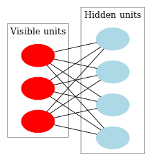
A DBN can be efficiently trained in an unsupervised, layer-by-layer manner, where the layers are typically made of restricted Boltzmann machines (RBM). An RBM is an undirected, generative energy-based model with a "visible" input layer and a hidden layer, and connections between the layers but not within layers. The training method for RBMs proposed by Geoffrey Hinton for use with training "Product of Expert" models is called contrastive divergence (CD).^[143] CD provides an approximation to the maximum likelihood method that would ideally be applied for learning the weights of the RBM.^[123]^[144] In training a single RBM, weight updates are performed with gradient ascent via the following equation: $\Delta w_{ij}(t+1)=w_{ij}(t)+\eta {\frac {\partial \log(p(v))}{\partial w_{ij}}}$ . Here, $p(v)$ is the probability of a visible vector, which is given by $p(v)={\frac {1}{Z}}\sum _{h}e^{-E(v,h)}$ . $Z$ is the partition function (used for normalizing) and $E(v,h)$ is the energy function assigned to the state of the network. A lower energy indicates the network is in a more "desirable" configuration. The gradient ${\frac {\partial \log(p(v))}{\partial w_{ij}}}$ has the simple form $\langle v_{i}h_{j}\rangle _{\text{data}}-\langle v_{i}h_{j}\rangle _{\text{model}}$ where $\langle \cdots \rangle _{p}$ represent averages with respect to distribution $p$ . The issue arises in sampling $\langle v_{i}h_{j}\rangle _{\text{model}}$ because this requires running alternating Gibbs sampling for a long time. CD replaces this step by running alternating Gibbs sampling for $n$ steps (values of $n=1$ have empirically been shown to perform well). After $n$ steps, the data are sampled and that sample is used in place of $\langle v_{i}h_{j}\rangle _{\text{model}}$ . The CD procedure works as follows:^[123]

Initialize the visible units to a training vector.
Update the hidden units in parallel given the visible units: $p(h_{j}=1\mid {\textbf {V}})=\sigma (b_{j}+\sum _{i}v_{i}w_{ij})$ . $\sigma$ is the sigmoid function and $b_{j}$ is the bias of $h_{j}$ .
Update the visible units in parallel given the hidden units: $p(v_{i}=1\mid {\textbf {H}})=\sigma (a_{i}+\sum _{j}h_{j}w_{ij})$ . $a_{i}$ is the bias of $v_{i}$ . This is called the "reconstruction" step.
Re-update the hidden units in parallel given the reconstructed visible units using the same equation as in step 2.
Perform the weight update: $\Delta w_{ij}\propto \langle v_{i}h_{j}\rangle _{\text{data}}-\langle v_{i}h_{j}\rangle _{\text{reconstruction}}$ .

Once an RBM is trained, another RBM is "stacked" atop it, taking its input from the final already-trained layer. The new visible layer is initialized to a training vector, and values for the units in the already-trained layers are assigned using the current weights and biases. The new RBM is then trained with the procedure above. This whole process is repeated until some desired stopping criterion is met.^[3]

Although the approximation of CD to maximum likelihood is very crude ( has been shown to not follow the gradient of any function), it has been empirically shown to be effective in training deep architectures.^[123]

Convolutional deep belief networks

A recent achievement in deep learning is the use of convolutional deep belief networks (CDBN). CDBNs have structure very similar to a convolutional neural networks and are trained similar to deep belief networks. Therefore, they exploit the 2D structure of images, like CNNs do, and make use of pre-training like deep belief networks. They provide a generic structure which can be used in many image and signal processing tasks. Recently, many benchmark results on standard image datasets like CIFAR^[145] have been obtained using CDBNs.^[146]

Large memory storage and retrieval neural networks

Large memory storage and retrieval neural networks (LAMSTAR)^[147]^[148] are fast deep learning neural networks of many layers which can use many filters simultaneously. These filters may be nonlinear, stochastic, logic, non-stationary, or even non-analytical. They are biologically motivated and continuously learning.

A LAMSTAR neural network may serve as a dynamic neural network in spatial or time domain or both. Its speed is provided by Hebbian link-weights (Chapter 9 of in D. Graupe, 2013^[149]), which serve to integrate the various and usually different filters (preprocessing functions) into its many layers and to dynamically rank the significance of the various layers and functions relative to a given task for deep learning. This grossly imitates biological learning which integrates outputs various preprocessors (cochlea, retina, etc.) and cortexes (auditory, visual, etc.) and their various regions. Its deep learning capability is further enhanced by using inhibition, correlation and by its ability to cope with incomplete data, or "lost" neurons or layers even at the midst of a task. Furthermore, it is fully transparent due to its link weights. The link-weights also allow dynamic determination of innovation and redundancy, and facilitate the ranking of layers, of filters or of individual neurons relative to a task.

LAMSTAR has been applied to many medical^[150]^[151]^[152] and financial predictions (see Graupe, 2013^[153] Section 9C), adaptive filtering of noisy speech in unknown noise,^[154] still-image recognition^[155] (Graupe, 2013^[156] Section 9D), video image recognition,^[157] software security,^[158] adaptive control of non-linear systems,^[159] and others. LAMSTAR had a much faster computing speed and somewhat lower error than a convolutional neural network based on ReLU-function filters and max pooling, in a comparative character recognition study.^[160]

These applications demonstrate delving into aspects of the data that are hidden from shallow learning networks or even from the human senses (eye, ear), such as in the cases of predicting onset of sleep apnea events,^[151] of an electrocardiogram of a fetus as recorded from skin-surface electrodes placed on the mother's abdomen early in pregnancy,^[152] of financial prediction (Section 9C in Graupe, 2013),^[147] or in blind filtering of noisy speech.^[154]

LAMSTAR was proposed in 1996 (A U.S. Patent 5,920,852 A) and was further developed by D Graupe and H Kordylewski 1997-2002.^[161]^[162]^[163] A modified version, known as LAMSTAR 2, was developed by N C Schneider and D Graupe in 2008.^[164]^[165]

Deep Boltzmann machines

A deep Boltzmann machine (DBM) is a type of binary pairwise Markov random field (undirected probabilistic graphical model) with multiple layers of hidden random variables. It is a network of symmetrically coupled stochastic binary units. It comprises a set of visible units ${\boldsymbol {\nu }}\in \{0,1\}^{D}$ , and a series of layers of hidden units ${\boldsymbol {h}}^{(1)}\in \{0,1\}^{F_{1}},{\boldsymbol {h}}^{(2)}\in \{0,1\}^{F_{2}},\ldots ,{\boldsymbol {h}}^{(L)}\in \{0,1\}^{F_{L}}$ . There is no connection between units of the same layer (like RBM). For the DBM, the probability assigned to vector $ν$ is

p({\boldsymbol {\nu }})={\frac {1}{Z}}\sum _{h}e^{\sum _{ij}W_{ij}^{(1)}\nu _{i}h_{j}^{(1)}+\sum _{jl}W_{jl}^{(2)}h_{j}^{(1)}h_{l}^{(2)}+\sum _{lm}W_{lm}^{(3)}h_{l}^{(2)}h_{m}^{(3)}},

where ${\boldsymbol {h}}=\{{\boldsymbol {h}}^{(1)},{\boldsymbol {h}}^{(2)},{\boldsymbol {h}}^{(3)}\}$ are the set of hidden units, and $\theta =\{{\boldsymbol {W}}^{(1)},{\boldsymbol {W}}^{(2)},{\boldsymbol {W}}^{(3)}\}$ are the model parameters, representing visible-hidden and hidden-hidden interactions. If ${\boldsymbol {W}}^{(2)}=0$ and ${\boldsymbol {W}}^{(3)}=0$ the network is the well-known restricted Boltzmann machine.^[166] Interactions are symmetric because links are undirected. By contrast, in a deep belief network (DBN) only the top two layers form a restricted Boltzmann machine (which is an undirected graphical model), but lower layers form a directed generative model.

Like DBNs, DBMs can learn complex and abstract internal representations of the input in tasks such as object or speech recognition, using limited labeled data to fine-tune the representations built using a large supply of unlabeled sensory input data. However, unlike DBNs and deep convolutional neural networks, they adopt the inference and training procedure in both directions, bottom-up and top-down pass, which allow the DBMs to better unveil the representations of the ambiguous and complex input structures.^[167]^[168]

However, the speed of DBMs limits their performance and functionality. Because exact maximum likelihood learning is intractable for DBMs, we may perform approximate maximum likelihood learning. Another option is to use mean-field inference to estimate data-dependent expectations, and approximation the expected sufficient statistics of the model by using Markov chain Monte Carlo (MCMC).^[166] This approximate inference, which must be done for each test input, is about 25 to 50 times slower than a single bottom-up pass in DBMs. This makes the joint optimization impractical for large data sets, and seriously restricts the use of DBMs for tasks such as feature representation.^[169]

Stacked (de-noising) auto-encoders

The auto encoder idea is motivated by the concept of a good representation. For example, for a classifier, a good representation can be defined as one that will yield a better performing classifier.

An encoder is a deterministic mapping $f_{\theta }$ that transforms an input vector x into hidden representation y, where $\theta =\{{\boldsymbol {W}},b\}$ , ${\boldsymbol {W}}$ is the weight matrix and b is an offset vector (bias). A decoder maps back the hidden representation y to the reconstructed input z via $g_{\theta }$ . The whole process of auto encoding is to compare this reconstructed input to the original and try to minimize this error to make the reconstructed value as close as possible to the original.

In stacked denoising auto encoders, the partially corrupted output is cleaned (de-noised). This idea was introduced in 2010 by Vincent et al.^[170] with a specific approach to good representation, a good representation is one that can be obtained robustly from a corrupted input and that will be useful for recovering the corresponding clean input. Implicit in this definition are the following ideas:

The higher level representations are relatively stable and robust to input corruption;
It is necessary to extract features that are useful for representation of the input distribution.

The algorithm consists of multiple steps; starts by a stochastic mapping of ${\boldsymbol {x}}$ to ${\tilde {\boldsymbol {x}}}$ through $q_{D}({\tilde {\boldsymbol {x}}}|{\boldsymbol {x}})$ , this is the corrupting step. Then the corrupted input ${\tilde {\boldsymbol {x}}}$ passes through a basic auto encoder process and is mapped to a hidden representation ${\boldsymbol {y}}=f_{\theta }({\tilde {\boldsymbol {x}}})=s({\boldsymbol {W}}{\tilde {\boldsymbol {x}}}+b)$ . From this hidden representation, we can reconstruct ${\boldsymbol {z}}=g_{\theta }({\boldsymbol {y}})$ . In the last stage, a minimization algorithm runs in order to have z as close as possible to uncorrupted input ${\boldsymbol {x}}$ . The reconstruction error $L_{H}({\boldsymbol {x}},{\boldsymbol {z}})$ might be either the cross-entropy loss with an affine-sigmoid decoder, or the squared error loss with an affine decoder.^[170]

In order to make a deep architecture, auto encoders stack one on top of another.^[171] Once the encoding function $f_{\theta }$ of the first denoising auto encoder is learned and used to uncorrupt the input (corrupted input), we can train the second level.^[170]

Once the stacked auto encoder is trained, its output can be used as the input to a supervised learning algorithm such as support vector machine classifier or a multi-class logistic regression.^[170]

Deep stacking networks

One deep architecture based on a hierarchy of blocks of simplified neural network modules is a deep convex network, introduced in 2011.^[172] Here, the weights learning problem is formulated as a convex optimization problem with a closed-form solution. This architecture is also called a deep stacking network (DSN),^[173] emphasizing the mechanism's similarity to stacked generalization.^[174] Each DSN block is a simple module that is easy to train by itself in a supervised fashion without back-propagation for the entire blocks.^[175]

As designed by Deng and Dong,^[172] each block consists of a simplified multi-layer perceptron (MLP) with a single hidden layer. The hidden layer h has logistic sigmoidal units, and the output layer has linear units. Connections between these layers are represented by weight matrix U; input-to-hidden-layer connections have weight matrix W. Target vectors t form the columns of matrix T, and the input data vectors x form the columns of matrix X. The matrix of hidden units is ${\boldsymbol {H}}=\sigma ({\boldsymbol {W}}^{T}{\boldsymbol {X}})$ . Modules are trained in order, so lower-layer weights W are known at each stage. The function performs the element-wise logistic sigmoid operation. Each block estimates the same final label class y, and its estimate is concatenated with original input X to form the expanded input for the next block. Thus, the input to the first block contains the original data only, while downstream blocks' input also has the output of preceding blocks. Then learning the upper-layer weight matrix U given other weights in the network can be formulated as a convex optimization problem:

\min _{U^{T}}f=||{\boldsymbol {U}}^{T}{\boldsymbol {H}}-{\boldsymbol {T}}||_{F}^{2},

which has a closed-form solution.

Unlike other deep architectures, such as DBNs, the goal is not to discover the transformed feature representation. The structure of the hierarchy of this kind of architecture makes parallel learning straightforward, as a batch-mode optimization problem. In purely discriminative tasks, DSNs perform better than conventional DBN.^[173]

Tensor deep stacking networks

This architecture is an extension of deep stacking networks (DSN). It improves on DSN in two important ways: it uses higher-order information from covariance statistics, and it transforms the non-convex problem of a lower-layer to a convex sub-problem of an upper-layer.^[176] TDSNs use covariance statistics of the data by using a bilinear mapping from each of two distinct sets of hidden units in the same layer to predictions, via a third-order tensor.

While parallelization and scalability are not considered seriously in conventional DNNs,^[177]^[178]^[179] all learning for DSNs and TDSNs is done in batch mode, to allow parallelization on a cluster of CPU or GPU nodes.^[172]^[173] Parallelization allows scaling the design to larger (deeper) architectures and data sets.

The basic architecture is suitable for diverse tasks such as classification and regression.

Spike-and-slab RBMs

The need for deep learning with real-valued inputs, as in Gaussian restricted Boltzmann machines, motivates the spike-and-slab RBM (ssRBMs), which models continuous-valued inputs with strictly binary latent variables.^[180] Similar to basic RBMs and its variants, a spike-and-slab RBM is a bipartite graph, while like GRBMs, the visible units (input) are real-valued. The difference is in the hidden layer, where each hidden unit has a binary spike variable and a real-valued slab variable. A spike is a discrete probability mass at zero, while a slab is a density over continuous domain;^[181]^[181] their mixture forms a prior. The terms come from the statistics literature.^[182]

An extension of ssRBM called µ-ssRBM provides extra modeling capacity using additional terms in the energy function. One of these terms enables the model to form a conditional distribution of the spike variables by marginalizing out the slab variables given an observation.

Compound hierarchical-deep models

Compound hierarchical-deep models compose deep networks with non-parametric Bayesian models. Features can be learned using deep architectures such as DBNs,^[90] DBMs,^[167] deep auto encoders,^[183] convolutional variants,^[184]^[185] ssRBMs,^[181] deep coding networks,^[186] DBNs with sparse feature learning,^[187] recursive neural networks,^[188] conditional DBNs,^[189] de-noising auto encoders.^[190] This provides a better representation, allowing faster learning and more accurate classification with high-dimensional data. However, these architectures are poor at learning novel classes with few examples, because all network units are involved in representing the input (a distributed representation) and must be adjusted together (high degree of freedom). Limiting the degree of freedom reduces the number of parameters to learn, facilitating learning of new classes from few examples. Hierarchical Bayesian (HB) models allow learning from few examples, for example^[191]^[192]^[193]^[194]^[195] for computer vision, statistics, and cognitive science.

Compound HD architectures aim to integrate characteristics of both HB and deep networks. The compound HDP-DBM architecture, a hierarchical Dirichlet process (HDP) as a hierarchical model, incorporated with DBM architecture. It is a full generative model, generalized from abstract concepts flowing through the layers of the model, which is able to synthesize new examples in novel classes that look reasonably natural. All the levels are learned jointly by maximizing a joint log-probability score.^[196]

In a DBM with three hidden layers, the probability of a visible input $ν$ is:

p({\boldsymbol {\nu }},\psi )={\frac {1}{Z}}\sum _{h}e^{\sum _{ij}W_{ij}^{(1)}\nu _{i}h_{j}^{1}+\sum _{jl}W_{jl}^{(2)}h_{j}^{1}h_{l}^{2}+\sum _{lm}W_{lm}^{(3)}h_{l}^{2}h_{m}^{3}},

where ${\boldsymbol {h}}=\{{\boldsymbol {h}}^{(1)},{\boldsymbol {h}}^{(2)},{\boldsymbol {h}}^{(3)}\}$ is the set of hidden units, and $\psi =\{{\boldsymbol {W}}^{(1)},{\boldsymbol {W}}^{(2)},{\boldsymbol {W}}^{(3)}\}$ are the model parameters, representing visible-hidden and hidden-hidden symmetric interaction terms.

After a DBM model is learned, we have an undirected model that defines the joint distribution $P(\nu ,h^{1},h^{2},h^{3})$ . One way to express what has been learned is the conditional model $P(\nu ,h^{1},h^{2}|h^{3})$ and a prior term $P(h^{3})$ .

Here $P(\nu ,h^{1},h^{2}|h^{3})$ represents a conditional DBM model, which can be viewed as a two-layer DBM but with bias terms given by the states of $h^{3}$ :

P(\nu ,h^{1},h^{2}|h^{3})={\frac {1}{Z(\psi ,h^{3})}}e^{\sum _{ij}W_{ij}^{(1)}\nu _{i}h_{j}^{1}+\sum _{jl}W_{jl}^{(2)}h_{j}^{1}h_{l}^{2}+\sum _{lm}W_{lm}^{(3)}h_{l}^{2}h_{m}^{3}}.

Deep coding networks

There are advantages of a model which can actively update itself from the context in data. Deep coding network (DPCN) is a predictive coding scheme where top-down information is used to empirically adjust the priors needed for a bottom-up inference procedure by means of a deep locally connected generative model. This works by extracting sparse features from time-varying observations using a linear dynamical model. Then, a pooling strategy is used to learn invariant feature representations. These units compose to form a deep architecture, and are trained by greedy layer-wise unsupervised learning. The layers constitute a kind of Markov chain such that the states at any layer only depend on the preceding and succeeding layers.

Deep predictive coding network (DPCN)^[197] predicts the representation of the layer, by using a top-down approach using the information in upper layer and temporal dependencies from the previous states.

DPCNs can be extended to form a convolutional network.^[197]

Deep Q-networks

A deep Q-network (DQN) is a type of deep learning model developed at Google DeepMind which combines a deep convolutional neural network with Q-learning, a form of reinforcement learning. Unlike earlier reinforcement learning agents, DQNs can learn directly from high-dimensional sensory inputs. Preliminary results were presented in 2014, with a paper published in February 2015 in Nature^[198] The application discussed in this paper is limited to Atari 2600 gaming, although it has implications for other applications. However, much before this work, there had been a number of reinforcement learning models that apply deep learning approaches (e.g.,^[199]).

Networks with separate memory structures

Integrating external memory with artificial neural networks dates to early research in distributed representations^[200] and Teuvo Kohonen's self-organizing maps. For example, in sparse distributed memory or hierarchical temporal memory, the patterns encoded by neural networks are used as addresses for content-addressable memory, with "neurons" essentially serving as address encoders and decoders. However, the early controllers of such memories were not differentiable.

LSTM-related differentiable memory structures

Apart from long short-term memory (LSTM), other approaches of the 1990s and 2000s also added differentiable memory to recurrent functions. For example:

Differentiable push and pop actions for alternative memory networks called neural stack machines^[201]^[202]
Memory networks where the control network's external differentiable storage is in the fast weights of another network^[203]
LSTM "forget gates"^[204]
Self-referential recurrent neural networks (RNNs) with special output units for addressing and rapidly manipulating each of the RNN's own weights in differentiable fashion (internal storage)^[205]^[206]
Learning to transduce with unbounded memory^[207]

Semantic hashing

Approaches which represent previous experiences directly and use a similar experience to form a local model are often called nearest neighbour or k-nearest neighbors methods.^[208] More recently, deep learning was shown to be useful in semantic hashing^[209] where a deep graphical model the word-count vectors^[210] obtained from a large set of documents. Documents are mapped to memory addresses in such a way that semantically similar documents are located at nearby addresses. Documents similar to a query document can then be found by simply accessing all the addresses that differ by only a few bits from the address of the query document. Unlike sparse distributed memory which operates on 1000-bit addresses, semantic hashing works on 32 or 64-bit addresses found in a conventional computer architecture.

Neural Turing machines

Neural Turing machines,^[211] developed by Google DeepMind, couple LSTM networks to external memory resources, which they can interact with by attentional processes. The combined system is analogous to a Turing machine but is differentiable end-to-end, allowing it to be efficiently trained by gradient descent. Preliminary results demonstrate that neural Turing machines can infer simple algorithms such as copying, sorting, and associative recall from input and output examples.

Memory networks

Memory networks^[212]^[213] are another extension to neural networks incorporating long-term memory, which was developed by the Facebook research team. The long-term memory can be read and written to, with the goal of using it for prediction. These models have been applied in the context of question answering (QA) where the long-term memory effectively acts as a (dynamic) knowledge base, and the output is a textual response.^[214]

Pointer networks

Deep neural networks can be potentially improved if they get deeper and have fewer parameters, while maintaining trainability. While training extremely deep (e.g. 1-million-layer-deep) neural networks might not be practically feasible, CPU-like architectures such as pointer networks^[215] and neural random-access machines^[216] developed by Google Brain researchers overcome this limitation by using external random-access memory as well as adding other components that typically belong to a computer architecture such as registers, ALU and pointers. Such systems operate on probability distribution vectors stored in memory cells and registers. Thus, the model is fully differentiable and trains end-to-end. The key characteristic of these models is that their depth, the size of their short-term memory, and the number of parameters can be altered independently — unlike models like Long short-term memory, whose number of parameters grows quadratically with memory size.

Encoder–decoder networks

An encoder–decoder framework is a framework based on neural networks that aims to map highly structured input to highly structured output. It was proposed recently in the context of machine translation,^[217]^[218]^[219] where the input and output are written sentences in two natural languages. In that work, an LSTM recurrent neural network (RNN) or convolutional neural network (CNN) was used as an encoder to summarize a source sentence, and the summary was decoded using a conditional recurrent neural network language model to produce the translation.^[220] All these systems have the same building blocks: gated RNNs and CNNs, and trained attention mechanisms.

Other architectures

Multilayer kernel machine

Multilayer kernel machines (MKM) as introduced in ^[221] are a way of learning highly nonlinear functions by iterative application of weakly nonlinear kernels. They use the kernel principal component analysis (KPCA), in ^[222] as method for unsupervised greedy layer-wise pre-training step of the deep learning architecture.

Layer $l+1$ -th learns the representation of the previous layer $l$ , extracting the $n_{l}$ principal component (PC) of the projection layer $l$ output in the feature domain induced by the kernel. For the sake of dimensionality reduction of the updated representation in each layer, a supervised strategy is proposed to select the best informative features among features extracted by KPCA. The process is:

rank the $n_{l}$ features according to their mutual information with the class labels;
for different values of K and $m_{l}\in \{1,\ldots ,n_{l}\}$ , compute the classification error rate of a K-nearest neighbor (K-NN) classifier using only the $m_{l}$ most informative features on a validation set;
the value of $m_{l}$ with which the classifier has reached the lowest error rate determines the number of features to retain.

There are some drawbacks in using the KPCA method as the building cells of an MKM.

A more straightforward way to use kernel machines for deep learning was developed by Microsoft researchers for spoken language understanding.^[223] The main idea is to use a kernel machine to approximate a shallow neural net with an infinite number of hidden units, then use stacking to splice the output of the kernel machine and the raw input in building the next, higher level of the kernel machine. The number of levels in the deep convex network is a hyper-parameter of the overall system, to be determined by cross validation.

Applications

Automatic speech recognition

Main article: Speech recognition

Speech recognition has been revolutionised by deep learning, especially by Long short-term memory (LSTM), a recurrent neural network published by Sepp Hochreiter & Jürgen Schmidhuber in 1997.^[52] LSTM RNNs circumvent the vanishing gradient problem and can learn "Very Deep Learning" tasks^[5] that involve speech events separated by thousands of discrete time steps, where one time step corresponds to about 10 ms. In 2003, LSTM with forget gates^[106] became competitive with traditional speech recognizers on certain tasks.^[53] In 2007, LSTM trained by Connectionist Temporal Classification (CTC)^[54] achieved excellent results in certain applications,^[55] although computers were much slower than today. In 2015, Google's large scale speech recognition suddenly almost doubled its performance through CTC-trained LSTM, now available to all smartphone users.^[56]

The initial success of deep learning in speech recognition, however, was based on small-scale TIMIT tasks. The results shown in the table below are for automatic speech recognition on the popular TIMIT data set. This is a common data set used for initial evaluations of deep learning architectures. The entire set contains 630 speakers from eight major dialects of American English, where each speaker reads 10 sentences.^[224] Its small size allows many configurations to be tried effectively. More importantly, the TIMIT task concerns phone-sequence recognition, which, unlike word-sequence recognition, allows very weak "language models" and thus the weaknesses in acoustic modeling aspects of speech recognition can be more easily analyzed. Such analysis on TIMIT by Li Deng and collaborators around 2009-2010, contrasting the GMM (and other generative models of speech) vs. DNN models, stimulated early industrial investment in deep learning for speech recognition from small to large scales,^[49]^[70] eventually leading to pervasive and dominant use in that industry. That analysis was done with comparable performance (less than 1.5% in error rate) between discriminative DNNs and generative models. The error rates listed below, including these early results and measured as percent phone error rates (PER), have been summarized over a time span of the past 20 years:

Method	PER (%)
Randomly Initialized RNN	26.1
Bayesian Triphone GMM-HMM	25.6
Hidden Trajectory (Generative) Model	24.8
Monophone Randomly Initialized DNN	23.4
Monophone DBN-DNN	22.4
Triphone GMM-HMM with BMMI Training	21.7
Monophone DBN-DNN on fbank	20.7
Convolutional DNN^[225]	20.0
Convolutional DNN w. Heterogeneous Pooling	18.7
Ensemble DNN/CNN/RNN^[226]	18.2
Bidirectional LSTM	17.9

In 2010, industrial researchers extended deep learning from TIMIT to large vocabulary speech recognition, by adopting large output layers of the DNN based on context-dependent HMM states constructed by decision trees.^[227]^[228]^[229] Comprehensive reviews of this development and of the state of the art as of October 2014 are provided in the recent Springer book from Microsoft Research.^[71] An earlier article^[230] reviewed the background of automatic speech recognition and the impact of various machine learning paradigms, including deep learning.

One fundamental principle of deep learning is to do away with hand-crafted feature engineering and to use raw features. This principle was first explored successfully in the architecture of deep autoencoder on the "raw" spectrogram or linear filter-bank features at SRI in the late 1990s,^[47] and later at Microsoft,^[231] showing its superiority over the Mel-Cepstral features which contain a few stages of fixed transformation from spectrograms. The true "raw" features of speech, waveforms, have more recently been shown to produce excellent larger-scale speech recognition results.^[232]

Since the initial successful debut of DNNs for speaker recognition in the late 1990s and speech recognition around 2009-2011 and of LSTM around 2003-2007, there have been huge new progresses made. Progress (and future directions) can be summarized into eight major areas:^[2]^[51]^[71]

Scaling up/out and speedup DNN training and decoding;
Sequence discriminative training of DNNs;
Feature processing by deep models with solid understanding of the underlying mechanisms;
Adaptation of DNNs and of related deep models;
Multi-task and transfer learning by DNNs and related deep models;
Convolution neural networks and how to design them to best exploit domain knowledge of speech;
Recurrent neural network and its rich LSTM variants;
Other types of deep models including tensor-based models and integrated deep generative/discriminative models.

Large-scale automatic speech recognition is the first and most convincing successful case of deep learning in the recent history, embraced by both industry and academia across the board. Between 2010 and 2014, the two major conferences on signal processing and speech recognition, IEEE-ICASSP and Interspeech, have seen a large increase in the numbers of accepted papers in their respective annual conference papers on the topic of deep learning for speech recognition. More importantly, all major commercial speech recognition systems (e.g., Microsoft Cortana, Xbox, Skype Translator, Amazon Alexa, Google Now, Apple Siri, Baidu and iFlyTek voice search, and a range of Nuance speech products, etc.) are all based on deep learning methods.^[2]^[233]^[234]^[235] See also the recent media interview with the CTO of Nuance Communications.^[236]

Image recognition

A common evaluation set for image classification is the MNIST database data set. MNIST is composed of handwritten digits and includes 60,000 training examples and 10,000 test examples. As with TIMIT, its small size allows multiple configurations to be tested. A comprehensive list of results on this set can be found in.^[237] The current best result on MNIST is an error rate of 0.23%, achieved by Ciresan et al. in 2012.^[238]

According to LeCun,^[68] in the early 2000s, in an industrial application CNNs already processed an estimated 10% to 20% of all the checks written in the US in the early 2000s. Significant additional impact of deep learning in image or object recognition was felt in the years 2011–2012. Although CNNs trained by backpropagation had been around for decades,^[33] and GPU implementations of NNs for years,^[73] including CNNs,^[74] fast implementations of CNNs with max-pooling on GPUs in the style of Dan Ciresan and colleagues^[94] were needed to make a dent in computer vision.^[5] In 2011, this approach achieved for the first time superhuman performance in a visual pattern recognition contest.^[96] Also in 2011, it won the ICDAR Chinese handwriting contest, and in May 2012, it won the ISBI image segmentation contest.^[97] Until 2011, CNNs did not play a major role at computer vision conferences, but in June 2012, a paper by Dan Ciresan et al. at the leading conference CVPR^[99] showed how max-pooling CNNs on GPU can dramatically improve many vision benchmark records, sometimes with human-competitive or even superhuman performance. In October 2012, a similar system by Alex Krizhevsky in the team of Geoff Hinton^[98] won the large-scale ImageNet competition by a significant margin over shallow machine learning methods. In November 2012, Ciresan et al.'s system also won the ICPR contest on analysis of large medical images for cancer detection, and in the following year also the MICCAI Grand Challenge on the same topic.^[239] In 2013 and 2014, the error rate on the ImageNet task using deep learning was further reduced quickly, following a similar trend in large-scale speech recognition.

As in the ambitious moves from automatic speech recognition toward automatic speech translation and understanding, image classification has recently been extended to the more challenging task of automatic image captioning, in which deep learning (often as a combination of CNNs and LSTMs) is the essential underlying technology^[240]^[241]^[242]^[243]

One example application is a car computer said to be trained with deep learning, which may enable cars to interpret 360° camera views.^[244] Another example is the technology known as Facial Dysmorphology Novel Analysis (FDNA) used to analyze cases of human malformation connected to a large database of genetic syndromes.

Natural language processing

Neural networks have been used for implementing language models since the early 2000s.^[107]^[245] Recurrent neural networks, especially LSTM,^[52] are most appropriate for sequential data such as language. LSTM helped to improve machine translation^[108] and Language Modeling.^[109]^[110] LSTM combined with CNNs also improved automatic image captioning^[141] and a plethora of other applications.^[5]

Other key techniques in this field are negative sampling^[246] and word embedding. Word embedding, such as word2vec, can be thought of as a representational layer in a deep learning architecture, that transforms an atomic word into a positional representation of the word relative to other words in the dataset; the position is represented as a point in a vector space. Using word embedding as an input layer to a recursive neural network (RNN) allows the training of the network to parse sentences and phrases using an effective compositional vector grammar. A compositional vector grammar can be thought of as probabilistic context free grammar (PCFG) implemented by a recursive neural network.^[247] Recursive auto-encoders built atop word embeddings have been trained to assess sentence similarity and detect paraphrasing.^[247] Deep neural architectures have achieved state-of-the-art results in many natural language processing tasks such as constituency parsing,^[248] sentiment analysis,^[249] information retrieval,^[250]^[251] spoken language understanding,^[252] machine translation,^[108]^[253] contextual entity linking,^[254] and others.^[255]

Drug discovery and toxicology

The pharmaceutical industry faces the problem that a large percentage of candidate drugs fail to reach the market. These failures of chemical compounds are caused by insufficient efficacy on the biomolecular target (on-target effect), undetected and undesired interactions with other biomolecules (off-target effects), or unanticipated toxic effects.^[256]^[257] In 2012, a team led by George Dahl won the "Merck Molecular Activity Challenge" using multi-task deep neural networks to predict the biomolecular target of a compound.^[258]^[259] In 2014, Sepp Hochreiter's group used Deep Learning to detect off-target and toxic effects of environmental chemicals in nutrients, household products and drugs and won the "Tox21 Data Challenge" of NIH, FDA and NCATS.^[260]^[261] These impressive successes show that deep learning may be superior to other virtual screening methods.^[262]^[263] Researchers from Google and Stanford enhanced deep learning for drug discovery by combining data from a variety of sources.^[264] In 2015, Atomwise introduced AtomNet, the first deep learning neural networks for structure-based rational drug design.^[265] Subsequently, AtomNet was used to predict novel candidate biomolecules for several disease targets, most notably treatments for the Ebola virus^[266] and multiple sclerosis.^[267]^[268]

Customer relationship management

Recently success has been reported with application of deep reinforcement learning in direct marketing settings, illustrating suitability of the method for CRM automation. A neural network was used to approximate the value of possible direct marketing actions over the customer state space, defined in terms of RFM variables. The estimated value function was shown to have a natural interpretation as customer lifetime value.^[269]

Recommendation systems

Recommendation systems have used deep learning to extract meaningful deep features for latent factor model for content-based recommendation for music.^[270] Recently, a more general approach for learning user preferences from multiple domains using multiview deep learning has been introduced.^[271] The model uses a hybrid collaborative and content-based approach and enhances recommendations in multiple tasks.

Biomedical Informatics

Recently, a deep-learning approach based on an autoencoder artificial neural network has been used in bioinformatics, to predict Gene Ontology annotations and gene-function relationships.^[272]

In medical informatics, deep learning has also been used in the health domain, including the prediction of sleep quality based on wearable data ^[273] and predictions of health complications from Electronic Health Record data.^[274]

Theories of the human brain

Computational deep learning is closely related to a class of theories of brain development (specifically, neocortical development) proposed by cognitive neuroscientists in the early 1990s.^[275] An approachable summary of this work is Elman, et al.'s 1996 book "Rethinking Innateness"^[276] (see also: Shrager and Johnson;^[277] Quartz and Sejnowski^[278]). As these developmental theories were also instantiated in computational models, they are technical predecessors of purely computationally motivated deep learning models. These developmental models share the interesting property that various proposed learning dynamics in the brain (e.g., a wave of nerve growth factor) conspire to support the self-organization of just the sort of inter-related neural networks utilized in the later, purely computational deep learning models; and such computational neural networks seem analogous to a view of the brain's neocortex as a hierarchy of filters in which each layer captures some of the information in the operating environment, and then passes the remainder, as well as modified base signal, to other layers further up the hierarchy. This process yields a self-organizing stack of transducers, well-tuned to their operating environment. As described in The New York Times in 1995: "...the infant's brain seems to organize itself under the influence of waves of so-called trophic-factors ... different regions of the brain become connected sequentially, with one layer of tissue maturing before another and so on until the whole brain is mature."^[279]

The importance of deep learning with respect to the evolution and development of human cognition did not escape the attention of these researchers. One aspect of human development that distinguishes us from our nearest primate neighbors may be changes in the timing of development.^[280] Among primates, the human brain remains relatively plastic until late in the post-natal period, whereas the brains of our closest relatives are more completely formed by birth. Thus, humans have greater access to the complex experiences afforded by being out in the world during the most formative period of brain development. This may enable us to "tune in" to rapidly changing features of the environment that other animals, more constrained by evolutionary structuring of their brains, are unable to take account of. To the extent that these changes are reflected in similar timing changes in hypothesized wave of cortical development, they may also lead to changes in the extraction of information from the stimulus environment during the early self-organization of the brain. Of course, along with this flexibility comes an extended period of immaturity, during which we are dependent upon our caretakers and our community for both support and training. The theory of deep learning therefore sees the coevolution of culture and cognition as a fundamental condition of human evolution.^[281]

Commercial activities

Deep learning is often presented as a step towards realising strong AI^[282] and thus many organizations have become interested in its use for particular applications. In December 2013, Facebook hired Yann LeCun to head its new artificial intelligence (AI) lab that was to have operations in California, London, and New York. The AI lab will develop deep learning techniques to help Facebook do tasks such as automatically tagging uploaded pictures with the names of the people in them.^[283] Late in 2014, Facebook also hired Vladimir Vapnik, a main developer of the Vapnik–Chervonenkis theory of statistical learning, and co-inventor of the support vector machine method.^[284]

In 2014, Google also bought DeepMind Technologies, a British start-up that developed a system capable of learning how to play Atari video games using only raw pixels as data input. In 2015 they demonstrated AlphaGo system which achieved one of the long-standing "grand challenges" of AI by learning the game of Go well enough to beat a human professional Go player.^[285]^[286]^[287]

In 2015, Blippar demonstrated a new mobile augmented reality application that makes use of deep learning to recognize objects in real time.^[288]

Criticism and comment

Given the far-reaching implications of artificial intelligence coupled with the realization that deep learning is emerging as one of its most powerful techniques, the subject is understandably attracting both criticism and comment, and in some cases from outside the field of computer science itself.

A main criticism of deep learning concerns the lack of theory surrounding many of the methods. Learning in the most common deep architectures is implemented using gradient descent; while gradient descent has been understood for a while now, the theory surrounding other algorithms, such as contrastive divergence is less clear. (i.e., Does it converge? If so, how fast? What is it approximating?) Deep learning methods are often looked at as a black box, with most confirmations done empirically, rather than theoretically.

Others point out that deep learning should be looked at as a step towards realizing strong AI, not as an all-encompassing solution. Despite the power of deep learning methods, they still lack much of the functionality needed for realizing this goal entirely. Research psychologist Gary Marcus has noted that:

"Realistically, deep learning is only part of the larger challenge of building intelligent machines. Such techniques lack ways of representing causal relationships (...) have no obvious ways of performing logical inferences, and they are also still a long way from integrating abstract knowledge, such as information about what objects are, what they are for, and how they are typically used. The most powerful A.I. systems, like Watson (...) use techniques like deep learning as just one element in a very complicated ensemble of techniques, ranging from the statistical technique of Bayesian inference to deductive reasoning."^[289]

To the extent that such a viewpoint implies, without intending to, that deep learning will ultimately constitute nothing more than the primitive discriminatory levels of a comprehensive future machine intelligence, a recent pair of speculations regarding art and artificial intelligence^[290] offers an alternative and more expansive outlook. The first such speculation is that it might be possible to train a machine vision stack to perform the sophisticated task of discriminating between "old master" and amateur figure drawings; and the second is that such a sensitivity might in fact represent the rudiments of a non-trivial machine empathy. It is suggested, moreover, that such an eventuality would be in line with anthropology, which identifies a concern with aesthetics as a key element of behavioral modernity (e.g., in ^[291]).

In further reference to the idea that a significant degree of artistic sensitivity might inhere within relatively low levels, whether biological or digital, of the cognitive hierarchy, a published series of graphic representations of the internal states of deep (20-30 layers) neural networks attempting to discern within essentially random data the images on which they were trained^[292] seem to demonstrate a striking visual appeal in light of the remarkable level of public attention which this work captured: the original research notice received well over 1,000 comments, and the The Guardian coverage^[293] was for a time the most frequently accessed article on that newspaper's web site.

Some currently popular and successful deep learning architectures display certain problematic behaviors,^[294] such as confidently classifying unrecognizable images as belonging to a familiar category of ordinary images^[295] and misclassifying minuscule perturbations of correctly classified images.^[296] The creator of OpenCog, Ben Goertzel, hypothesized^[294] that these behaviors are due to limitations in the internal representations learned by these architectures, and that these limitations would inhibit integration of these architectures into heterogeneous multi-component AGI architectures. It is suggested that these issues can be worked around by developing deep learning architectures that internally form states homologous to image-grammar^[297] decompositions of observed entities and events.^[294] Learning a grammar (visual or linguistic) from training data would be equivalent to restricting the system to commonsense reasoning which operates on concepts in terms of production rules of the grammar, and is a basic goal of both human language acquisition^[298] and AI. (See also Grammar induction.^[299])

Software libraries

Main article: Comparison of deep learning software

Deeplearning4j — An open-source deep-learning library written for Java/C++ with LSTMs and convolutional networks. It provides parallelization with Spark on CPUs and GPUs.
Gensim — A toolkit for natural language processing implemented in the Python programming language.
Keras — An open-source deep learning framework for the Python programming language.
Microsoft CNTK (Computational Network Toolkit) — Microsoft's open-source deep-learning toolkit for Windows and Linux. It provides parallelization with CPUs and GPUs across multiple servers.
OpenNN — An open source C++ library which implements deep neural networks and provides parallelization with CPUs.
PaddlePaddle — An open source C++ /CUDA library with Python API for scalable deep learning platform with CPUs and GPUs, originally developed by Baidu.
TensorFlow — Google's open source machine learning library in C++ and Python with APIs for both. It provides parallelization with CPUs and GPUs.
Theano — An open source machine learning library for Python supported by the University of Montreal and Yoshua Bengio's team.
Torch — An open source software library for machine learning based on the Lua programming language and used by Facebook.

References

↑ Ian Goodfellow, Yoshua Bengio, and Aaron Courville (2016). Deep Learning. MIT Press. Online
1 2 3 4 5 6 7 8 9 Deng, L.; Yu, D. (2014). "Deep Learning: Methods and Applications" (PDF). Foundations and Trends in Signal Processing. 7 (3-4): 1–199. doi:10.1561/2000000039.
1 2 3 4 5 6 7 Bengio, Yoshua (2009). "Learning Deep Architectures for AI" (PDF). Foundations and Trends in Machine Learning. 2 (1): 1–127. doi:10.1561/2200000006.
1 2 3 4 5 6 Bengio, Y.; Courville, A.; Vincent, P. (2013). "Representation Learning: A Review and New Perspectives". IEEE Transactions on Pattern Analysis and Machine Intelligence. 35 (8): 1798–1828. arXiv:1206.5538. doi:10.1109/tpami.2013.50.
1 2 3 4 5 6 7 8 9 10 11 12 13 14 15 16 17 18 Schmidhuber, J. (2015). "Deep Learning in Neural Networks: An Overview". Neural Networks. 61: 85–117. arXiv:1404.7828. doi:10.1016/j.neunet.2014.09.003.
↑ Bengio, Yoshua; LeCun, Yann; Hinton, Geoffrey (2015). "Deep Learning". Nature. 521: 436–444. doi:10.1038/nature14539.
↑ Deep Machine Learning – A New Frontier in Artificial Intelligence Research – a survey paper by Itamar Arel, Derek C. Rose, and Thomas P. Karnowski. IEEE Computational Intelligence Magazine, 2013
1 2 3 4 5 6 7 Schmidhuber, Jürgen (2015). "Deep Learning". Scholarpedia. 10 (11): 32832. doi:10.4249/scholarpedia.32832.
↑ Carlos E. Perez. "A Pattern Language for Deep Learning".
↑ Glauner, P. (2015). Deep Convolutional Neural Networks for Smile Recognition (MSc Thesis). Imperial College London, Department of Computing. arXiv:1508.06535.
↑ Song, H.A.; Lee, S. Y. (2013). "Hierarchical Representation Using NMF". Neural Information Processing. Lectures Notes in Computer Sciences. 8226. Springer Berlin Heidelberg. pp. 466–473. doi:10.1007/978-3-642-42054-2_58. ISBN 978-3-642-42053-5.
↑ Olshausen, B. A. (1996). "Emergence of simple-cell receptive field properties by learning a sparse code for natural images". Nature. 381 (6583): 607–609. doi:10.1038/381607a0.
↑ Collobert, R. (April 2011). Deep Learning for Efficient Discriminative Parsing. VideoLectures.net. Event occurs at 7min 45s.
↑ Gomes, L. (20 October 2014). "Machine-Learning Maestro Michael Jordan on the Delusions of Big Data and Other Huge Engineering Efforts". IEEE Spectrum.
↑ Deep learning classes at Google, etc.
1 2 Rina Dechter (1986). Learning while searching in constraint-satisfaction problems. University of California, Computer Science Department, Cognitive Systems Laboratory.Online
1 2 3 4 5 6 7 J. Schmidhuber., "Learning complex, extended sequences using the principle of history compression," Neural Computation, 4, pp. 234–242, 1992.
1 2 3 4 Hinton, G.E. "Deep belief networks". Scholarpedia. 4 (5): 5947. doi:10.4249/scholarpedia.5947.
1 2 Balázs Csanád Csáji. Approximation with Artificial Neural Networks; Faculty of Sciences; Eötvös Loránd University, Hungary
1 2 3 Cybenko (1989). "Approximations by superpositions of sigmoidal functions" (PDF). Mathematics of Control, Signals, and Systems. 2 (4): 303–314. doi:10.1007/bf02551274.
1 2 3 Hornik, Kurt (1991). "Approximation Capabilities of Multilayer Feedforward Networks". Neural Networks. 4 (2): 251–257. doi:10.1016/0893-6080(91)90009-t.
1 2 Haykin, Simon (1998). Neural Networks: A Comprehensive Foundation, Volume 2, Prentice Hall. ISBN 0-13-273350-1.
1 2 Hassoun, M. (1995) Fundamentals of Artificial Neural Networks MIT Press, p. 48
1 2 3 4 Murphy, K.P. (2012) Machine learning: a probabilistic perspective MIT Press
↑ Hinton, G. E.; Srivastava, N.; Krizhevsky, A.; Sutskever, I.; Salakhutdinov, R.R. (2012). "Improving neural networks by preventing co-adaptation of feature detectors". arXiv:1207.0580 [math.LG].
1 2 Ivakhnenko, Alexey (1965). Cybernetic Predicting Devices. Kiev: Naukova Dumka.
1 2 3 Ivakhnenko, Alexey (1971). "Polynomial theory of complex systems". IEEE Transactions on Systems, Man and Cybernetics (4): 364–378.
1 2 Fukushima, K. (1980). "Neocognitron: A self-organizing neural network model for a mechanism of pattern recognition unaffected by shift in position". Biol. Cybern. 36: 193–202. doi:10.1007/bf00344251.
1 2 3 4 Seppo Linnainmaa (1970). The representation of the cumulative rounding error of an algorithm as a Taylor expansion of the local rounding errors. Master's Thesis (in Finnish), Univ. Helsinki, 6-7.
1 2 Griewank, Andreas (2012). Who Invented the Reverse Mode of Differentiation?. Optimization Stories, Documenta Matematica, Extra Volume ISMP (2012), 389-400.
1 2 P. Werbos., "Beyond Regression: New Tools for Prediction and Analysis in the Behavioral Sciences," PhD thesis, Harvard University, 1974.
1 2 3 Paul Werbos (1982). Applications of advances in nonlinear sensitivity analysis. In System modeling and optimization (pp. 762-770). Springer Berlin Heidelberg. Online
1 2 3 LeCun et al., "Backpropagation Applied to Handwritten Zip Code Recognition," Neural Computation, 1, pp. 541–551, 1989.
1 2 Jürgen Schmidhuber (1993). Habilitation thesis, TUM, 1993. Page 150 ff demonstrates credit assignment across the equivalent of 1,200 layers in an unfolded RNN. Online
↑ Hinton, Geoffrey E.; Dayan, Peter; Frey, Brendan J.; Neal, Radford (1995-05-26). "The wake-sleep algorithm for unsupervised neural networks". Science. 268 (5214): 1158–1161. doi:10.1126/science.7761831.
1 2 3 4 5 S. Hochreiter., "Untersuchungen zu dynamischen neuronalen Netzen," Diploma thesis. Institut f. Informatik, Technische Univ. Munich. Advisor: J. Schmidhuber, 1991.
1 2 S. Hochreiter et al., "Gradient flow in recurrent nets: the difficulty of learning long-term dependencies," In S. C. Kremer and J. F. Kolen, editors, A Field Guide to Dynamical Recurrent Neural Networks. IEEE Press, 2001.
1 2 3 4 J. Weng, N. Ahuja and T. S. Huang, "Cresceptron: a self-organizing neural network which grows adaptively," Proc. International Joint Conference on Neural Networks, Baltimore, Maryland, vol I, pp. 576-581, June, 1992.
1 2 3 4 5 J. Weng, N. Ahuja and T. S. Huang, "Learning recognition and segmentation of 3-D objects from 2-D images," Proc. 4th International Conf. Computer Vision, Berlin, Germany, pp. 121-128, May, 1993.
1 2 3 4 J. Weng, N. Ahuja and T. S. Huang, "Learning recognition and segmentation using the Cresceptron," International Journal of Computer Vision, vol. 25, no. 2, pp. 105-139, Nov. 1997.
↑ Morgan, Bourlard, Renals, Cohen, Franco (1993) "Hybrid neural network/hidden Markov model systems for continuous speech recognition. ICASSP/IJPRAI"
↑ T. Robinson. (1992) A real-time recurrent error propagation network word recognition system, ICASSP.
↑ Waibel, Hanazawa, Hinton, Shikano, Lang. (1989) "Phoneme recognition using time-delay neural networks. IEEE Transactions on Acoustics, Speech and Signal Processing."
↑ Baker, J.; Deng, Li; Glass, Jim; Khudanpur, S.; Lee, C.-H.; Morgan, N.; O'Shaughnessy, D. (2009). "Research Developments and Directions in Speech Recognition and Understanding, Part 1". IEEE Signal Processing Magazine. 26 (3): 75–80. doi:10.1109/msp.2009.932166.
↑ Y. Bengio (1991). "Artificial Neural Networks and their Application to Speech/Sequence Recognition," Ph.D. thesis, McGill University, Canada.
↑ Deng, L.; Hassanein, K.; Elmasry, M. (1994). "Analysis of correlation structure for a neural predictive model with applications to speech recognition". Neural Networks. 7 (2): 331–339. doi:10.1016/0893-6080(94)90027-2.
1 2 Heck, L.; Konig, Y.; Sonmez, M.; Weintraub, M. (2000). "Robustness to Telephone Handset Distortion in Speaker Recognition by Discriminative Feature Design". Speech Communication. 31 (2): 181–192. doi:10.1016/s0167-6393(99)00077-1.
1 2 3 Hinton, G.; Deng, L.; Yu, D.; Dahl, G.; Mohamed, A.; Jaitly, N.; Senior, A.; Vanhoucke, V.; Nguyen, P.; Sainath, T.; Kingsbury, B. (2012). "Deep Neural Networks for Acoustic Modeling in Speech Recognition --- The shared views of four research groups". IEEE Signal Processing Magazine. 29 (6): 82–97. doi:10.1109/msp.2012.2205597.
1 2 3 Deng, L.; Hinton, G.; Kingsbury, B. (2013). "New types of deep neural network learning for speech recognition and related applications: An overview (ICASSP)".
1 2 Keynote talk: Recent Developments in Deep Neural Networks. ICASSP, 2013 (by Geoff Hinton).
1 2 Keynote talk: "Achievements and Challenges of Deep Learning - From Speech Analysis and Recognition To Language and Multimodal Processing," Interspeech, September 2014.
1 2 3 4 5 6 7 8 Hochreiter, Sepp; and Schmidhuber, Jürgen; Long Short-Term Memory, Neural Computation, 9(8):1735–1780, 1997
1 2 3 Alex Graves, Douglas Eck, Nicole Beringer, and Jürgen Schmidhuber (2003). Biologically Plausible Speech Recognition with LSTM Neural Nets. 1st Intl. Workshop on Biologically Inspired Approaches to Advanced Information Technology, Bio-ADIT 2004, Lausanne, Switzerland, p. 175-184, 2004. Online
1 2 3 4 5 Alex Graves, Santiago Fernandez, Faustino Gomez, and Jürgen Schmidhuber (2006). Connectionist temporal classification: Labelling unsegmented sequence data with recurrent neural nets. Proceedings of ICML’06, pp. 369–376.
1 2 3 4 Santiago Fernandez, Alex Graves, and Jürgen Schmidhuber (2007). An application of recurrent neural networks to discriminative keyword spotting. Proceedings of ICANN (2), pp. 220–229.
1 2 3 4 5 Haşim Sak, Andrew Senior, Kanishka Rao, Françoise Beaufays and Johan Schalkwyk (September 2015): Google voice search: faster and more accurate.
↑ Igor Aizenberg, Naum N. Aizenberg, Joos P.L. Vandewalle (2000). Multi-Valued and Universal Binary Neurons: Theory, Learning and Applications. Springer Science & Business Media.
↑ Google Ngram chart of the usage of the expression "deep learning" posted by Jürgen Schmidhuber (2015) Online
↑ G. E. Hinton., "Learning multiple layers of representation," Trends in Cognitive Sciences, 11, pp. 428–434, 2007.
↑ J. Schmidhuber., "My First Deep Learning System of 1991 + Deep Learning Timeline 1962–2013." Online
↑ http://research.microsoft.com/apps/pubs/default.aspx?id=189004
↑ L. Deng et al. Recent Advances in Deep Learning for Speech Research at Microsoft, ICASSP, 2013.
↑ L. Deng, O. Abdel-Hamid, and D. Yu, A deep convolutional neural network using heterogeneous pooling for trading acoustic invariance with phonetic confusion, ICASSP, 2013.
1 2 T. Sainath et al., "Convolutional neural networks for LVCSR," ICASSP, 2013.
1 2 Hasim Sak and Andrew Senior and Francoise Beaufays (2014). Long Short-Term Memory recurrent neural network architectures for large scale acoustic modeling. Proceedings of Interspeech 2014.
1 2 Xiangang Li, Xihong Wu (2015). Constructing Long Short-Term Memory based Deep Recurrent Neural Networks for Large Vocabulary Speech Recognition arXiv:1410.4281
1 2 Heiga Zen and Hasim Sak (2015). Unidirectional Long Short-Term Memory Recurrent Neural Network with Recurrent Output Layer for Low-Latency Speech Synthesis. In Proceedings of ICASSP, pp. 4470-4474.
1 2 3 Yann LeCun (2016). Slides on Deep Learning Online
↑ D. Yu, L. Deng, G. Li, and F. Seide (2011). "Discriminative pretraining of deep neural networks," U.S. Patent Filing.
1 2 NIPS Workshop: Deep Learning for Speech Recognition and Related Applications, Whistler, BC, Canada, Dec. 2009 (Organizers: Li Deng, Geoff Hinton, D. Yu).
1 2 3 Yu, D.; Deng, L. (2014). "Automatic Speech Recognition: A Deep Learning Approach (Publisher: Springer)".
↑ IEEE (2015)http://blogs.technet.com/b/inside_microsoft_research/archive/2015/12/03/deng-receives-prestigious-ieee-technical-achievement-award.aspx
1 2 Oh, K.-S.; Jung, K. (2004). "GPU implementation of neural networks". Pattern Recognition. 37 (6): 1311–1314. doi:10.1016/j.patcog.2004.01.013.
1 2 Chellapilla, K., Puri, S., and Simard, P. (2006). High performance convolutional neural networks for document processing. International Workshop on Frontiers in Handwriting Recognition.
1 2 D. C. Ciresan et al., "Deep Big Simple Neural Nets for Handwritten Digit Recognition," Neural Computation, 22, pp. 3207–3220, 2010.
↑ R. Raina, A. Madhavan, A. Ng., "Large-scale Deep Unsupervised Learning using Graphics Processors," Proc. 26th Int. Conf. on Machine Learning, 2009.
↑ Riesenhuber, M; Poggio, T (1999). "Hierarchical models of object recognition in cortex". Nature Neuroscience. 2 (11): 1019–1025. doi:10.1038/14819.
↑ Y. LeCun, B. Boser, J. S. Denker, D. Henderson, R. E. Howard, W. Hubbard, L. D. Jackel. 1989 Backpropagation Applied to Handwritten Zip Code Recognition. Neural Computation, 1(4):541–551.
1 2 3 Griewank, Andreas and Walther, A.. Principles and Techniques of Algorithmic Differentiation, Second Edition. SIAM, 2008.
1 2 Henry J. Kelley (1960). Gradient theory of optimal flight paths. Ars Journal, 30(10), 947-954. Online
1 2 Arthur E. Bryson (1961, April). A gradient method for optimizing multi-stage allocation processes. In Proceedings of the Harvard Univ. Symposium on digital computers and their applications.
1 2 Stuart Dreyfus (1962). The numerical solution of variational problems. Journal of Mathematical Analysis and Applications, 5(1), 30-45. Online
1 2 Stuart Dreyfus (1973). The computational solution of optimal control problems with time lag. IEEE Transactions on Automatic Control, 18(4):383–385.
1 2 Rumelhart, D. E., Hinton, G. E. & Williams, R. J. , "Learning representations by back-propagating errors" nature, 1974.
1 2 Stuart Dreyfus (1990). Artificial Neural Networks, Back Propagation and the Kelley-Bryson Gradient Procedure. J. Guidance, Control and Dynamics, 1990.
1 2 Graves, Alex; and Schmidhuber, Jürgen; Offline Handwriting Recognition with Multidimensional Recurrent Neural Networks, in Bengio, Yoshua; Schuurmans, Dale; Lafferty, John; Williams, Chris K. I.; and Culotta, Aron (eds.), Advances in Neural Information Processing Systems 22 (NIPS'22), December 7th–10th, 2009, Vancouver, BC, Neural Information Processing Systems (NIPS) Foundation, 2009, pp. 545–552
↑ Graves, A.; Liwicki, M.; Fernandez, S.; Bertolami, R.; Bunke, H.; Schmidhuber, J. (2009). "A Novel Connectionist System for Improved Unconstrained Handwriting Recognition". IEEE Transactions on Pattern Analysis and Machine Intelligence. 31 (5): 855–868. doi:10.1109/tpami.2008.137.
↑ Sven Behnke (2003). Hierarchical Neural Networks for Image Interpretation. (PDF). Lecture Notes in Computer Science. 2766. Springer.
↑ Smolensky, P. (1986). "Information processing in dynamical systems: Foundations of harmony theory.". In D. E. Rumelhart, J. L. McClelland, & the PDP Research Group. Parallel Distributed Processing: Explorations in the Microstructure of Cognition. 1. pp. 194–281.
1 2 Hinton, G. E.; Osindero, S.; Teh, Y. (2006). "A fast learning algorithm for deep belief nets" (PDF). Neural Computation. 18 (7): 1527–1554. doi:10.1162/neco.2006.18.7.1527. PMID 16764513.
↑ Hinton, G. (2009). "Deep belief networks". Scholarpedia. 4 (5): 5947. doi:10.4249/scholarpedia.5947.
↑ John Markoff (25 June 2012). "How Many Computers to Identify a Cat? 16,000.". New York Times.
↑ Ng, Andrew; Dean, Jeff (2012). "Building High-level Features Using Large Scale Unsupervised Learning". arXiv:1112.6209.
1 2 3 D. C. Ciresan, U. Meier, J. Masci, L. M. Gambardella, J. Schmidhuber. Flexible, High Performance Convolutional Neural Networks for Image Classification. International Joint Conference on Artificial Intelligence (IJCAI-2011, Barcelona), 2011.
↑ Martines, H.; Bengio, Y.; Yannakakis, G. N. (2013). "Learning Deep Physiological Models of Affect". IEEE Computational Intelligence. 8 (2): 20–33. doi:10.1109/mci.2013.2247823.
1 2 D. C. Ciresan, U. Meier, J. Masci, J. Schmidhuber. Multi-Column Deep Neural Network for Traffic Sign Classification. Neural Networks, 2012.
1 2 D. Ciresan, A. Giusti, L. Gambardella, J. Schmidhuber. Deep Neural Networks Segment Neuronal Membranes in Electron Microscopy Images. In Advances in Neural Information Processing Systems (NIPS 2012), Lake Tahoe, 2012.
1 2 Krizhevsky, A., Sutskever, I. and Hinton, G. E. (2012). ImageNet Classification with Deep Convolutional Neural Networks. NIPS 2012: Neural Information Processing Systems, Lake Tahoe, Nevada
1 2 D. C. Ciresan, U. Meier, J. Schmidhuber. Multi-column Deep Neural Networks for Image Classification. IEEE Conf. on Computer Vision and Pattern Recognition CVPR 2012.
↑ D. J. Felleman and D. C. Van Essen, "Distributed hierarchical processing in the primate cerebral cortex," Cerebral Cortex, 1, pp. 1-47, 1991.
↑ J. Weng, "Natural and Artificial Intelligence: Introduction to Computational Brain-Mind," BMI Press, ISBN 978-0985875725, 2012.
↑ J. Weng, "Why Have We Passed `Neural Networks Do not Abstract Well'?," Natural Intelligence: the INNS Magazine, vol. 1, no.1, pp. 13-22, 2011.
↑ Z. Ji, J. Weng, and D. Prokhorov, "Where-What Network 1: Where and What Assist Each Other Through Top-down Connections," Proc. 7th International Conference on Development and Learning (ICDL'08), Monterey, CA, Aug. 9-12, pp. 1-6, 2008.
↑ X. Wu, G. Guo, and J. Weng, "Skull-closed Autonomous Development: WWN-7 Dealing with Scales," Proc. International Conference on Brain-Mind, July 27–28, East Lansing, Michigan, pp. +1-9, 2013.
↑ Szegedy, Christian, Alexander Toshev, and Dumitru Erhan. "Deep neural networks for object detection." Advances in Neural Information Processing Systems. 2013.
1 2 3 Felix Gers, Nicholas Schraudolph, and Jürgen Schmidhuber (2002). Learning precise timing with LSTM recurrent networks. Journal of Machine Learning Research 3:115–143.
1 2 3 Felix A. Gers and Jürgen Schmidhuber. LSTM Recurrent Networks Learn Simple Context Free and Context Sensitive Languages. IEEE TNN 12(6):1333–1340, 2001.
1 2 3 4 I. Sutskever, O. Vinyals, Q. Le (2014) "Sequence to Sequence Learning with Neural Networks," Proc. NIPS.
1 2 3 Rafal Jozefowicz, Oriol Vinyals, Mike Schuster, Noam Shazeer, Yonghui Wu (2016). Exploring the Limits of Language Modeling. arXiv
1 2 3 Dan Gillick, Cliff Brunk, Oriol Vinyals, Amarnag Subramanya (2015). Multilingual Language Processing From Bytes. arXiv
↑ T. Mikolov et al., "Recurrent neural network based language model," Interspeech, 2010.
↑ LeCun, Y.; et al. "Gradient-based learning applied to document recognition". Proceedings of the IEEE. 86 (11): 2278–2324. doi:10.1109/5.726791.
↑ Eiji Mizutani, Stuart Dreyfus, Kenichi Nishio (2000). On derivation of MLP backpropagation from the Kelley-Bryson optimal-control gradient formula and its application. Proceedings of the IEEE International Joint Conference on Neural Networks (IJCNN 2000), Como Italy, July 2000. Online
↑ Bryson, A.E.; W.F. Denham; S.E. Dreyfus. Optimal programming problems with inequality constraints. I: Necessary conditions for extremal solutions. AIAA J. 1, 11 (1963) 2544-2550
↑ Stuart Russell; Peter Norvig. Artificial Intelligence A Modern Approach. p. 578. The most popular method for learning in multilayer networks is called Back-propagation.
↑ Arthur Earl Bryson, Yu-Chi Ho (1969). Applied optimal control: optimization, estimation, and control. Blaisdell Publishing Company or Xerox College Publishing. p. 481.
↑ Seppo Linnainmaa (1976). Taylor expansion of the accumulated rounding error. BIT Numerical Mathematics, 16(2), 146-160.
↑ Paul Werbos (1974). Beyond regression: New tools for prediction and analysis in the behavioral sciences. PhD thesis, Harvard University.
↑ Eric A. Wan (1993). Time series prediction by using a connectionist network with internal delay lines. In SANTA FE INSTITUTE STUDIES IN THE SCIENCES OF COMPLEXITY-PROCEEDINGS (Vol. 15, pp. 195-195). Addison-Wesley Publishing Co.
↑ G. E. Hinton et al.., "Deep Neural Networks for Acoustic Modeling in Speech Recognition: The shared views of four research groups," IEEE Signal Processing Magazine, pp. 82–97, November 2012.
↑ Y. Bengio et al.., "Advances in optimizing recurrent networks," ICASSP, 2013.
↑ G. Dahl et al.., "Improving DNNs for LVCSR using rectified linear units and dropout," ICASSP, 2013.
1 2 3 4 G. E. Hinton., "A Practical Guide to Training Restricted Boltzmann Machines," Tech. Rep. UTML TR 2010-003, Dept. CS., Univ. of Toronto, 2010.
↑ Huang, Guang-Bin; Zhu, Qin-Yu; Siew, Chee-Kheong (2006). "Extreme learning machine: theory and applications". Neurocomputing. 70 (1): 489–501. doi:10.1016/j.neucom.2005.12.126.
↑ Widrow, Bernard; et al. (2013). "The no-prop algorithm: A new learning algorithm for multilayer neural networks". Neural Networks. 37: 182–188. doi:10.1016/j.neunet.2012.09.020.
↑ Ollivier, Yann; Charpiat, Guillaume (2015). "Training recurrent networks without backtracking". arXiv:1507.07680.
↑ Aleksander, Igor, et al. "A brief introduction to Weightless Neural Systems." ESANN. 2009.
↑ Alexey Grigorevich Ivakhnenko and V. G. Lapa and R. N. McDonough (1967). Cybernetics and forecasting techniques. American Elsevier, NY.
↑ Alexey Grigorevich Ivakhnenko (1968). The group method of data handling – a rival of the method of stochastic approximation. Soviet Automatic Control, 13(3):43–55.
↑ T. Kondo and J. Ueno (2008). Multi-layered GMDH-type neural network self-selecting optimum neural network architecture and its application to 3-dimensional medical image recognition of blood vessels. International Journal of Innovative Computing,Information and Control, 4(1):175–187.
↑ http://ufldl.stanford.edu/tutorial/supervised/ConvolutionalNeuralNetwork/
↑ Szegedy, Christian; Liu, Wei; Jia, Yangqing; Sermanet, Pierre; Reed, Scott; Anguelov, Dragomir; Erhan, Dumitru; Vanhoucke, Vincent; Rabinovich, Andrew (2014). "Going Deeper with Convolutions". Computing Research Repository. arXiv:1409.4842.
↑ Goller, C.; Küchler, A. "Learning task-dependent distributed representations by backpropagation through structure". Neural Networks, 1996., IEEE. doi:10.1109/ICNN.1996.548916.
↑ Socher, Richard; Lin, Cliff; Ng, Andrew Y.; Manning, Christopher D. "Parsing Natural Scenes and Natural Language with Recursive Neural Networks". The 28th International Conference on Machine Learning (ICML 2011).
↑ Socher, Richard; Perelygin, Alex; Y. Wu, Jean; Chuang, Jason; D. Manning, Christopher; Y. Ng, Andrew; Potts, Christopher. "Recursive Deep Models for Semantic Compositionality Over a Sentiment Treebank" (PDF). EMNLP 2013.
↑ Justin Bayer, Daan Wierstra, Julian Togelius, and Jürgen Schmidhuber (2009). Evolving memory cell structures for sequence learning. Proceedings of ICANN (2), pp. 755–764.
↑ Santiago Fernandez, Alex Graves, and Jürgen Schmidhuber (2007). Sequence labelling in structured domains with hierarchical recurrent neural networks. Proceedings of IJCAI.
↑ Awni Hannun, Carl Case, Jared Casper, Bryan Catanzaro, Greg Diamos, Erich Elsen, Ryan Prenger, Sanjeev Satheesh, Shubho Sengupta, Adam Coates, Andrew Ng (2014). Deep Speech: Scaling up end-to-end speech recognition. arXiv:1412.5567
↑ Fan, Y., Qian, Y., Xie, F., and Soong, F. K. (2014). TTS synthesis with bidirectional LSTM based recurrent neural networks. In Proceedings of Interspeech.
↑ Bo Fan, Lijuan Wang, Frank K. Soong, and Lei Xie (2015). Photo-Real Talking Head with Deep Bidirectional LSTM. In Proceedings of ICASSP 2015.
1 2 Oriol Vinyals, Alexander Toshev, Samy Bengio, and Dumitru Erhan (2015). Show and Tell: A Neural Image Caption Generator. arXiv
↑ Larochelle, H.; et al. "An empirical evaluation of deep architectures on problems with many factors of variation". Proc. 24th Int. Conf. Machine Learning. 2007: 473–480.
↑ G. E. Hinton., "Training Product of Experts by Minimizing Contrastive Divergence," Neural Computation, 14, pp. 1771–1800, 2002.
↑ Fischer, A.; Igel, C. (2014). "Training Restricted Boltzmann Machines: An Introduction" (PDF). Pattern Recognition. 47: 25–39. doi:10.1016/j.patcog.2013.05.025.
↑ Convolutional Deep Belief Networks on CIFAR-10
↑ Convolutional deep belief networks for scalable unsupervised learning of hierarchical representations
1 2 D. Graupe, "Principles of Artificial Neural Networks.3rd Edition", World Scientific Publishers, 2013.
↑ D. Graupe," Large memory storage and retrieval (LAMSTAR) network, US Patent 5920852 A", April 1996.
↑ D. Graupe, "Principles of Artificial Neural Networks.3rd Edition", World Scientific Publishers, 2013, pp.203-274.
↑ V. P. Nigam, D. Graupe, (2004),"A neural-network-based detection of epilepsy", Neurological Research, 26(1): 55-60.
1 2 Waxman, J.; Graupe, D.; Carley, C W. (2010). "Automated prediction of apnea and hypopnea, using a LAMSTAR artificial neural network". American Journal of Respiratory and Critical Care Medicine. 171 (7): 727–733.
1 2 Graupe, D.; Graupe, M. H.; Zhong, Y.; Jackson, R. K. (2008). "Blind adaptive filtering for non-invasive extraction of the fetal electrocardiogram and its non-stationarities". Proc. Inst. Mech Eng., UK, Part H: Journal of Engineering in Medicine. 222 (8): 1221–1234. doi:10.1243/09544119jeim417.
↑ D. Graupe, "Principles of Artificial Neural Networks.3rd Edition", World Scientific Publishers, 2013, pp.240-253.
1 2 Graupe, D.; Abon, J. (2002). "A Neural Network for Blind Adaptive Filtering of Unknown Noise from Speech". Intelligent Engineering Systems Through Artificial Neural Networks. 12: 683–688.
↑ Homayon, S. (2015). "Iris Recognition for Personal Identification Using LAMSTAR Neural Network". International Journal of Computer Science and Information Technology. 7 (1).
↑ D. Graupe, "Principles of Artificial Neural Networks.3rd Edition", World Scientific Publishers", 2013, pp.253-274.
↑ Girado, J. I.; Sandin, D. J.; DeFanti, T. A. (2003). "Real-time camera-based face detection using amodified LAMSTAR neural network system". Proc. SPIE 5015, Applications of Artificial Neural Networks in Image Processing VIII. doi:10.1117/12.477405.
↑ Venkatachalam, V; Selvan, S. (2007). "Intrusion Detection using an Improved Competitive Learning Lamstar Network". International Journal of Computer Science and Network Security. 7 (2): 255–263.
↑ D. Graupe, M. Smollack, (2007), "Control of unstable nonlinear and nonstationary systems using LAMSTAR neural networks", Proceedings of 10th IASTED on Intelligent Control, Sect.592, 141-144.
↑ D. Graupe, C. Contaldi, A. Sattiraju, (2015) "Comparison of Lamstar NN & Convolutional NN – Character Recognition".
↑ Graupe, H. Kordylewski (1996). "Network based on SOM (self-organizing-map) modules combined with statistical decision tools". Proc. IEEE 39th Midwest Conf. on Circuits and Systems. 1: 471–475.
↑ D, Graupe, H. Kordylewski, (1998), "A large memory storage and retrieval neural network for adaptive retrieval and diagnosis", International Journal of Software Engineering and Knowledge Engineering, 1998.
↑ Kordylewski, H.; Graupe, D; Liu, K. "A novel large-memory neural network as an aid in medical diagnosis applications". IEEE Transactions on Information Technology in Biomedicine. 5 (3): 202–209. doi:10.1109/4233.945291.
↑ Schneider, N.C.; Graupe (2008). "A modified LAMSTAR neural network and its applications". International journal of neural systems. 18 (4): 331–337. doi:10.1142/s0129065708001634.
↑ D. Graupe, "Principles of Artificial Neural Networks.3rd Edition", World Scientific Publishers, 2013, p.217.
1 2 Hinton, Geoffrey; Salakhutdinov, Ruslan (2012). "A better way to pretrain deep Boltzmann machines" (PDF). Advances in Neural. 3: 1–9.
1 2 Hinton, Geoffrey; Salakhutdinov, Ruslan (2009). "Efficient Learning of Deep Boltzmann Machines" (PDF). 3: 448–455.
↑ Bengio, Yoshua; LeCun, Yann (2007). "Scaling Learning Algorithms towards AI" (PDF). 1: 1–41.
↑ Larochelle, Hugo; Salakhutdinov, Ruslan (2010). "Efficient Learning of Deep Boltzmann Machines" (PDF): 693–700.
1 2 3 4 Vincent, Pascal; Larochelle, Hugo; Lajoie, Isabelle; Bengio, Yoshua; Manzagol, Pierre-Antoine (2010). "Stacked Denoising Autoencoders: Learning Useful Representations in a Deep Network with a Local Denoising Criterion". The Journal of Machine Learning Research. 11: 3371–3408.
↑ Dana H. Ballard (1987). Modular learning in neural networks. Proceedings of AAAI, pages 279–284.
1 2 3 Deng, Li; Yu, Dong (2011). "Deep Convex Net: A Scalable Architecture for Speech Pattern Classification" (PDF). Proceedings of the Interspeech: 2285–2288.
1 2 3 Deng, Li; Yu, Dong; Platt, John (2012). "Scalable stacking and learning for building deep architectures" (PDF). 2012 IEEE International Conference on Acoustics, Speech and Signal Processing (ICASSP): 2133–2136.
↑ David, Wolpert (1992). "Stacked generalization". Neural Networks. 5 (2): 241–259. doi:10.1016/S0893-6080(05)80023-1.
↑ Bengio, Yoshua (2009). "Learning deep architectures for AI". Foundations and Trends in Machine Learning. 2 (1): 1–127. doi:10.1561/2200000006.
↑ Hutchinson, Brian; Deng, Li; Yu, Dong (2012). "Tensor deep stacking networks". IEEE Transactions on Pattern Analysis and Machine Intelligence. 1–15: 1944–1957. doi:10.1109/tpami.2012.268.
↑ Hinton, Geoffrey; Salakhutdinov, Ruslan (2006). "Reducing the Dimensionality of Data with Neural Networks". Science. 313: 504–507. doi:10.1126/science.1127647. PMID 16873662.
↑ Dahl, G.; Yu, D.; Deng, L.; Acero, A. (2012). "Context-Dependent Pre-Trained Deep Neural Networks for Large-Vocabulary Speech Recognition". IEEE Transactions on Audio, Speech, and Language Processing. 20 (1): 30–42. doi:10.1109/tasl.2011.2134090.
↑ Mohamed, Abdel-rahman; Dahl, George; Hinton, Geoffrey (2012). "Acoustic Modeling Using Deep Belief Networks". IEEE Transactions on Audio, Speech, and Language Processing. 20 (1): 14–22. doi:10.1109/tasl.2011.2109382.
↑ Courville, Aaron; Bergstra, James; Bengio, Yoshua (2011). "A Spike and Slab Restricted Boltzmann Machine" (PDF). JMLR: Workshop and Conference Proceeding. 15: 233–241.
1 2 3 Courville, Aaron; Bergstra, James; Bengio, Yoshua (2011). "Unsupervised Models of Images by Spike-and-Slab RBMs". Proceedings of the 28th International Conference on Machine Learning (PDF). 10. pp. 1–8.
↑ Mitchell, T; Beauchamp, J (1988). "Bayesian Variable Selection in Linear Regression". Journal of the American Statistical Association. 83 (404): 1023–1032. doi:10.1080/01621459.1988.10478694.
↑ Larochelle, Hugo; Bengio, Yoshua; Louradour, Jerdme; Lamblin, Pascal (2009). "Exploring Strategies for Training Deep Neural Networks". The Journal of Machine Learning Research. 10: 1–40.
↑ Coates, Adam; Carpenter, Blake (2011). "Text Detection and Character Recognition in Scene Images with Unsupervised Feature Learning": 440–445.
↑ Lee, Honglak; Grosse, Roger (2009). "Convolutional deep belief networks for scalable unsupervised learning of hierarchical representations". Proceedings of the 26th Annual International Conference on Machine Learning: 1–8.
↑ Lin, Yuanqing; Zhang, Tong (2010). "Deep Coding Network" (PDF). Advances in Neural . . .: 1–9.
↑ Ranzato, Marc Aurelio; Boureau, Y-Lan (2007). "Sparse Feature Learning for Deep Belief Networks" (PDF). Advances in Neural Information Processing Systems. 23: 1–8.
↑ Socher, Richard; Lin, Clif (2011). "Parsing Natural Scenes and Natural Language with Recursive Neural Networks" (PDF). Proceedings of the 26th International Conference on Machine Learning.
↑ Taylor, Graham; Hinton, Geoffrey (2006). "Modeling Human Motion Using Binary Latent Variables" (PDF). Advances in Neural Information Processing Systems.
↑ Vincent, Pascal; Larochelle, Hugo (2008). "Extracting and composing robust features with denoising autoencoders". Proceedings of the 25th international conference on Machine learning - ICML '08: 1096–1103.
↑ Kemp, Charles; Perfors, Amy; Tenenbaum, Joshua (2007). "Learning overhypotheses with hierarchical Bayesian models". Developmental Science. 10 (3): 307–21. doi:10.1111/j.1467-7687.2007.00585.x. PMID 17444972.
↑ Xu, Fei; Tenenbaum, Joshua (2007). "Word learning as Bayesian inference". Psychol. Rev. 114 (2): 245–72. doi:10.1037/0033-295X.114.2.245. PMID 17500627.
↑ Chen, Bo; Polatkan, Gungor (2011). "The Hierarchical Beta Process for Convolutional Factor Analysis and Deep Learning" (PDF). Machine Learning . . .
↑ Fei-Fei, Li; Fergus, Rob (2006). "One-shot learning of object categories". IEEE Transactions on Pattern Analysis and Machine Intelligence. 28 (4): 594–611. doi:10.1109/TPAMI.2006.79. PMID 16566508.
↑ Rodriguez, Abel; Dunson, David (2008). "The Nested Dirichlet Process". Journal of the American Statistical Association. 103 (483): 1131–1154. doi:10.1198/016214508000000553.
↑ Ruslan, Salakhutdinov; Joshua, Tenenbaum (2012). "Learning with Hierarchical-Deep Models". IEEE Transactions on Pattern Analysis and Machine Intelligence. 35: 1958–71. doi:10.1109/TPAMI.2012.269.
1 2 Chalasani, Rakesh; Principe, Jose (2013). "Deep Predictive Coding Networks". arXiv:1301.3541.
↑ Mnih, Volodymyr; et al. (2015). "Human-level control through deep reinforcement learning". Nature. 518: 529–533. doi:10.1038/nature14236. PMID 25719670.
↑ R. Sun and C. Sessions, Self-segmentation of sequences: Automatic formation of hierarchies of sequential behaviors. IEEE Transactions on Systems, Man, and Cybernetics: Part B Cybernetics, Vol.30, No.3, pp.403-418. 2000.
↑ Hinton, Geoffrey E. "Distributed representations." (1984)
↑ S. Das, C.L. Giles, G.Z. Sun, "Learning Context Free Grammars: Limitations of a Recurrent Neural Network with an External Stack Memory," Proc. 14th Annual Conf. of the Cog. Sci. Soc., p. 79, 1992.
↑ Mozer, M. C., & Das, S. (1993). A connectionist symbol manipulator that discovers the structure of context-free languages. NIPS 5 (pp. 863-870).
↑ Schmidhuber, J. (1992). "Learning to control fast-weight memories: An alternative to recurrent nets". Neural Computation. 4 (1): 131–139. doi:10.1162/neco.1992.4.1.131.
↑ Gers, F.; Schraudolph, N.; Schmidhuber, J. (2002). "Learning precise timing with LSTM recurrent networks". JMLR. 3: 115–143.
↑ Jürgen Schmidhuber (1993). "An introspective network that can learn to run its own weight change algorithm". In Proc. of the Intl. Conf. on Artificial Neural Networks, Brighton. IEE. pp. 191–195.
↑ Hochreiter, Sepp; Younger, A. Steven; Conwell, Peter R. (2001). "Learning to Learn Using Gradient Descent". ICANN. 2130: 87–94.
↑ Grefenstette, Edward, et al. "Learning to Transduce with Unbounded Memory." arXiv:1506.02516 (2015).
↑ Atkeson, Christopher G., and Stefan Schaal. "Memory-based neural networks for robot learning." Neurocomputing 9.3 (1995): 243-269.
↑ Salakhutdinov, Ruslan, and Geoffrey Hinton. "Semantic hashing." International Journal of Approximate Reasoning 50.7 (2009): 969-978.
↑ Le, Quoc V.; Mikolov, Tomas (2014). "Distributed representations of sentences and documents". arXiv:1405.4053.
↑ Graves, Alex, Greg Wayne, and Ivo Danihelka. "Neural Turing Machines." arXiv:1410.5401 (2014).
↑ Weston, Jason, Sumit Chopra, and Antoine Bordes. "Memory networks." arXiv:1410.3916 (2014).
↑ Sukhbaatar, Sainbayar, et al. "End-To-End Memory Networks." arXiv:1503.08895 (2015).
↑ Bordes, Antoine, et al. "Large-scale Simple Question Answering with Memory Networks." arXiv:1506.02075 (2015).
↑ Vinyals, Oriol, Meire Fortunato, and Navdeep Jaitly. "Pointer networks." arXiv:1506.03134 (2015).
↑ Kurach,Karol, Andrychowicz, Marcin and Sutskever,Ilya. "Neural Random-Access Machines." arXiv:1511.06392 (2015).
↑ N. Kalchbrenner and P. Blunsom, "Recurrent continuous translation models," in EMNLP’2013, 2013.
↑ I. Sutskever, O. Vinyals, and Q. V. Le, "Sequence to sequence learning with neural networks," in NIPS’2014, 2014.
↑ K. Cho, B. van Merrienboer, C. Gulcehre, F. Bougares, H. Schwenk, and Y. Bengio, "Learning phrase representations using RNN encoder-decoder for statistical machine translation," in Proceedings of the Empiricial Methods in Natural Language Processing (EMNLP 2014), Oct. 2014
↑ Cho, Kyunghyun, Aaron Courville, and Yoshua Bengio. "Describing Multimedia Content using Attention-based Encoder--Decoder Networks." arXiv:1507.01053 (2015).
↑ Cho, Youngmin (2012). "Kernel Methods for Deep Learning" (PDF): 1–9.
↑ Scholkopf, B; Smola, Alexander (1998). "Nonlinear component analysis as a kernel eigenvalue problem". Neural computation. (44): 1299–1319. doi:10.1162/089976698300017467.
↑ L. Deng, G. Tur, X. He, and D. Hakkani-Tur. "Use of Kernel Deep Convex Networks and End-To-End Learning for Spoken Language Understanding," Proc. IEEE Workshop on Spoken Language Technologies, 2012
↑ TIMIT Acoustic-Phonetic Continuous Speech Corpus Linguistic Data Consortium, Philadelphia.
↑ Abdel-Hamid, O.; et al. (2014). "Convolutional Neural Networks for Speech Recognition". IEEE/ACM Transactions on Audio, Speech, and Language Processing. 22 (10): 1533–1545. doi:10.1109/taslp.2014.2339736.
↑ Deng, L.; Platt, J. (2014). "Ensemble Deep Learning for Speech Recognition". Proc. Interspeech.
↑ Yu, D.; Deng, L. (2010). "Roles of Pre-Training and Fine-Tuning in Context-Dependent DBN-HMMs for Real-World Speech Recognition". NIPS Workshop on Deep Learning and Unsupervised Feature Learning.
↑ Seide, F., Li, G., Yu, D. Conversational speech transcription using context-dependent deep neural networks. Interspeech, 2011.
↑ Deng L., Li, J., Huang, J., Yao, K., Yu, D., Seide, F. et al. Recent Advances in Deep Learning for Speech Research at Microsoft. ICASSP, 2013.
↑ Deng, L.; Li, Xiao (2013). "Machine Learning Paradigms for Speech Recognition: An Overview". IEEE Transactions on Audio, Speech, and Language Processing. 21: 1060–1089. doi:10.1109/tasl.2013.2244083.
↑ L. Deng, M. Seltzer, D. Yu, A. Acero, A. Mohamed, and G. Hinton (2010) Binary Coding of Speech Spectrograms Using a Deep Auto-encoder. Interspeech.
↑ Z. Tuske, P. Golik, R. Schlüter and H. Ney (2014). Acoustic Modeling with Deep Neural Networks Using Raw Time Signal for LVCSR. Interspeech.
↑ McMillan, R. "How Skype Used AI to Build Its Amazing New Language Translator", Wire, Dec. 2014.
↑ Hannun et al. (2014) "Deep Speech: Scaling up end-to-end speech recognition", arXiv:1412.5567.
↑ "Plenary presentation at ICASSP-2016" (PDF).
↑ Ron Schneiderman (2015) "Accuracy, Apps Advance Speech Recognition --- Interviews with Vlad Sejnoha and Li Deng", IEEE Signal Processing Magazine, Jan, 2015.
↑ http://yann.lecun.com/exdb/mnist/.
↑ D. Ciresan, U. Meier, J. Schmidhuber., "Multi-column Deep Neural Networks for Image Classification," Technical Report No. IDSIA-04-12, 2012.
↑ D. Ciresan, A. Giusti, L.M. Gambardella, J. Schmidhuber (2013). Mitosis Detection in Breast Cancer Histology Images using Deep Neural Networks. Proceedings MICCAI, 2013.
↑ Vinyals et al. (2014)."Show and Tell: A Neural Image Caption Generator," arXiv:1411.4555.
↑ Fang et al. (2014)."From Captions to Visual Concepts and Back," arXiv:1411.4952.
↑ Kiros et al. (2014). "Unifying Visual-Semantic Embeddings with Multimodal Neural Language Models," arXiv:1411.2539.
↑ Zhong, S.; Liu, Y.; Liu, Y. "Bilinear Deep Learning for Image Classification". Proceedings of the 19th ACM International Conference on Multimedia. 11: 343–352.
↑ Nvidia Demos a Car Computer Trained with "Deep Learning" (2015-01-06), David Talbot, MIT Technology Review
↑ Y. Bengio, R. Ducharme, P. Vincent, C. Jauvin., "A Neural Probabilistic Language Model," Journal of Machine Learning Research 3 (2003) 1137–1155, 2003.
↑ Goldberg, Yoav; Levy, Omar. "word2vec Explained: Deriving Mikolov et al.'s Negative-Sampling Word-Embedding Method". arXiv:1402.3722.
1 2 Socher, Richard; Manning, Christopher. "Deep Learning for NLP" (PDF). Retrieved 26 October 2014.
↑ Socher, Richard; Bauer, John; Manning, Christopher; Ng, Andrew (2013). "Parsing With Compositional Vector Grammars" (PDF). Proceedings of the ACL 2013 conference.
↑ Socher, Richard (2013). "Recursive Deep Models for Semantic Compositionality Over a Sentiment Treebank" (PDF). EMNLP 2013.
↑ Y. Shen, X. He, J. Gao, L. Deng, and G. Mesnil (2014) " A Latent Semantic Model with Convolutional-Pooling Structure for Information Retrieval," Proc. CIKM.
↑ P. Huang, X. He, J. Gao, L. Deng, A. Acero, and L. Heck (2013) "Learning Deep Structured Semantic Models for Web Search using Clickthrough Data," Proc. CIKM.
↑ Mesnil, G., Dauphin, Y., Yao, K., Bengio, Y., Deng, L., Hakkani-Tur, D., He, X., Heck, L., Tur, G., Yu, D. and Zweig, G., 2015. Using recurrent neural networks for slot filling in spoken language understanding. IEEE Transactions on Audio, Speech, and Language Processing, 23(3), pp.530-539.
↑ J. Gao, X. He, W. Yih, and L. Deng(2014) "Learning Continuous Phrase Representations for Translation Modeling," Proc. ACL.
↑ J. Gao, P. Pantel, M. Gamon, X. He, L. Deng (2014) "Modeling Interestingness with Deep Neural Networks," Proc. EMNLP.
↑ J. Gao, X. He, L. Deng (2014) "Deep Learning for Natural Language Processing: Theory and Practice (Tutorial)," CIKM.
↑ Arrowsmith, J; Miller, P (2013). "Trial watch: Phase II and phase III attrition rates 2011-2012". Nature Reviews Drug Discovery. 12 (8): 569. doi:10.1038/nrd4090. PMID 23903212.
↑ Verbist, B; Klambauer, G; Vervoort, L; Talloen, W; The Qstar, Consortium; Shkedy, Z; Thas, O; Bender, A; Göhlmann, H. W.; Hochreiter, S (2015). "Using transcriptomics to guide lead optimization in drug discovery projects: Lessons learned from the QSTAR project". Drug Discovery Today. 20: 505–513. doi:10.1016/j.drudis.2014.12.014. PMID 25582842.
↑ "Announcement of the winners of the Merck Molecular Activity Challenge" https://www.kaggle.com/c/MerckActivity/details/winners.
↑ Dahl, G. E.; Jaitly, N.; & Salakhutdinov, R. (2014) "Multi-task Neural Networks for QSAR Predictions," ArXiv, 2014.
↑ "Toxicology in the 21st century Data Challenge" https://tripod.nih.gov/tox21/challenge/leaderboard.jsp
↑ "NCATS Announces Tox21 Data Challenge Winners" http://www.ncats.nih.gov/news-and-events/features/tox21-challenge-winners.html
↑ Unterthiner, T.; Mayr, A.; Klambauer, G.; Steijaert, M.; Ceulemans, H.; Wegner, J. K.; & Hochreiter, S. (2014) "Deep Learning as an Opportunity in Virtual Screening". Workshop on Deep Learning and Representation Learning (NIPS2014).
↑ Unterthiner, T.; Mayr, A.; Klambauer, G.; & Hochreiter, S. (2015) "Toxicity Prediction using Deep Learning". ArXiv, 2015.
↑ Ramsundar, B.; Kearnes, S.; Riley, P.; Webster, D.; Konerding, D.;& Pande, V. (2015) "Massively Multitask Networks for Drug Discovery". ArXiv, 2015.
↑ Wallach, Izhar; Dzamba, Michael; Heifets, Abraham (2015-10-09). "AtomNet: A Deep Convolutional Neural Network for Bioactivity Prediction in Structure-based Drug Discovery". arXiv:1510.02855.
↑ "Toronto startup has a faster way to discover effective medicines". The Globe and Mail. Retrieved 2015-11-09.
↑ "Startup Harnesses Supercomputers to Seek Cures". KQED Future of You. Retrieved 2015-11-09.
↑ http://www.theglobeandmail.com/report-on-business/small-business/starting-out/toronto-startup-has-a-faster-way-to-discover-effective-medicines/article25660419/%5d%20and%20multiple%20sclerosis%20%5b/
↑ Tkachenko, Yegor. Autonomous CRM Control via CLV Approximation with Deep Reinforcement Learning in Discrete and Continuous Action Space. (April 8, 2015). arXiv.org: http://arxiv.org/abs/1504.01840
↑ Van den Oord, Aaron, Sander Dieleman, and Benjamin Schrauwen. "Deep content-based music recommendation." Advances in Neural Information Processing Systems. 2013.
↑ Elkahky, Ali Mamdouh, Yang Song, and Xiaodong He. "A Multi-View Deep Learning Approach for Cross Domain User Modeling in Recommendation Systems." Proceedings of the 24th International Conference on World Wide Web. International World Wide Web Conferences Steering Committee, 2015.
↑ Davide Chicco, Peter Sadowski, and Pierre Baldi, "Deep autoencoder neural networks for gene ontology annotation predictions". Proceedings of the 5th ACM Conference on Bioinformatics, Computational Biology, and Health Informatics. ACM, 2014.
↑ Sathyanarayana, Aarti (2016-01-01). "Sleep Quality Prediction From Wearable Data Using Deep Learning". JMIR mHealth and uHealth. 4 (4). doi:10.2196/mhealth.6562.
↑ Choi, Edward; Schuetz, Andy; Stewart, Walter F.; Sun, Jimeng (2016-08-13). "Using recurrent neural network models for early detection of heart failure onset". Journal of the American Medical Informatics Association: ocw112. doi:10.1093/jamia/ocw112. ISSN 1067-5027. PMID 27521897.
↑ Utgoff, P. E.; Stracuzzi, D. J. (2002). "Many-layered learning". Neural Computation. 14: 2497–2529. doi:10.1162/08997660260293319.
↑ J. Elman et al., "Rethinking Innateness," 1996.
↑ Shrager, J.; Johnson, MH (1996). "Dynamic plasticity influences the emergence of function in a simple cortical array". Neural Networks. 9 (7): 1119–1129. doi:10.1016/0893-6080(96)00033-0.
↑ Quartz, SR; Sejnowski, TJ (1997). "The neural basis of cognitive development: A constructivist manifesto". Behavioral and Brain Sciences. 20 (4): 537–556. doi:10.1017/s0140525x97001581.
↑ S. Blakeslee., "In brain's early growth, timetable may be critical," The New York Times, Science Section, pp. B5–B6, 1995.
↑ {BUFILL} E. Bufill, J. Agusti, R. Blesa., "Human neoteny revisited: The case of synaptic plasticity," American Journal of Human Biology, 23 (6), pp. 729–739, 2011.
↑ J. Shrager and M. H. Johnson., "Timing in the development of cortical function: A computational approach," In B. Julesz and I. Kovacs (Eds.), Maturational windows and adult cortical plasticity, 1995.
↑ D. Hernandez., "The Man Behind the Google Brain: Andrew Ng and the Quest for the New AI," http://www.wired.com/wiredenterprise/2013/05/neuro-artificial-intelligence/all/. Wired, 10 May 2013.
↑ C. Metz., "Facebook's 'Deep Learning' Guru Reveals the Future of AI," http://www.wired.com/wiredenterprise/2013/12/facebook-yann-lecun-qa/. Wired, 12 December 2013.
↑ V. Vapnik., "research.facebook.com" .
↑ "Google AI algorithm masters ancient game of Go". Nature News & Comment. Retrieved 2016-01-30.
↑ Silver, David; Huang, Aja; Maddison, Chris J.; Guez, Arthur; Sifre, Laurent; van den Driessche, George; Schrittwieser, Julian; Antonoglou, Ioannis; Panneershelvam, Veda (2016-01-28). "Mastering the game of Go with deep neural networks and tree search". Nature. 529 (7587): 484–489. doi:10.1038/nature16961. ISSN 0028-0836.
↑ "A Google DeepMind Algorithm Uses Deep Learning and More to Master the Game of Go | MIT Technology Review". MIT Technology Review. Retrieved 2016-01-30.
↑ "Blippar Demonstrates New Real-Time Augmented Reality App". TechCrunch.
↑ G. Marcus., "Is "Deep Learning" a Revolution in Artificial Intelligence?" The New Yorker, 25 November 2012.
↑ Smith, G. W. (March 27, 2015). "Art and Artificial Intelligence". ArtEnt. Retrieved March 27, 2015.
↑ Knight, Will (November 7, 2001). "Tools point to African origin for human behaviour". New Scientist. Retrieved October 7, 2015.
↑ Alexander Mordvintsev; Christopher Olah; Mike Tyka (June 17, 2015). "Inceptionism: Going Deeper into Neural Networks". Google Research Blog. Retrieved June 20, 2015.
↑ Alex Hern (June 18, 2015). "Yes, androids do dream of electric sheep". The Guardian. Retrieved June 20, 2015.
1 2 3 Ben Goertzel. Are there Deep Reasons Underlying the Pathologies of Today's Deep Learning Algorithms? (2015) Url: http://goertzel.org/DeepLearning_v1.pdf
↑ Nguyen, Anh, Jason Yosinski, and Jeff Clune. "Deep Neural Networks are Easily Fooled: High Confidence Predictions for Unrecognizable Images." arXiv:1412.1897 (2014).
↑ Szegedy, Christian, et al. "Intriguing properties of neural networks." arXiv:1312.6199 (2013).
↑ Zhu, S.C.; Mumford, D. "A stochastic grammar of images". Found. Trends Comput. Graph. Vis. 2 (4): 259–362. doi:10.1561/0600000018.
↑ Miller, G. A., and N. Chomsky. "Pattern conception." Paper for Conference on pattern detection, University of Michigan. 1957.
↑ Jason Eisner, Deep Learning of Recursive Structure: Grammar Induction, http://techtalks.tv/talks/deep-learning-of-recursive-structure-grammar-induction/58089/

External links

This article is issued from Wikipedia - version of the 12/2/2016. The text is available under the Creative Commons Attribution/Share Alike but additional terms may apply for the media files.