Representation theory of the Lorentz group

Hendrik Antoon Lorentz (right) after whom the Lorentz group is named and Albert Einstein whose special theory of relativity is the main source of application. Photo taken by Paul Ehrenfest 1921.

The Lorentz group, a Lie group of symmetries of the spacetime of special relativity, has a wide variety of representations. The prominence of this representation theory is that in any relativistically invariant physical theory, representations of the Lorentz group must enter in some fashion,^{[nb 1]} by definition of relativistic invariance itself. Since special relativity together with quantum mechanics are the theories of which physicists are most certain,^{[nb 2]} this topic is of fundamental importance in theoretical physics.

Many of the representations, both finite-dimensional and infinite-dimensional, are important in the description of fields in classical field theory,^{[nb 3]} most importantly the electromagnetic field, and of particles in relativistic quantum mechanics,^{[nb 4]} as well as of both particles and quantum fields in quantum field theory^{[nb 5]} and of various objects in string theory^{[nb 6]} and beyond.^{[nb 7]} The representation theory also provides the theoretical ground for the concept of spin, which, for a particle, can be either integer or half-integer in the unit of the reduced Planck constant ℏ. Quantum mechanical wave functions representing particles with half-integer spin are called spinors. The classical electromagnetic field has spin as well. It transforms under a representation with spin one.^[1] The theory enters into general relativity in the sense that in small enough regions of spacetime, physics is that of special relativity.^[2] The group may also be represented in terms of a set of functions defined on the Riemann sphere. These are the Riemann P-functions, which are expressible as hypergeometric functions.

The identity component $SO(3; 1) +$ of the Lorentz group is isomorphic to the Möbius group, and hence any representation of the Lorentz group is necessarily a representation of the Möbius group and vice versa.The subgroup $SO(3)$ with its representation theory form a simpler theory, but the two are related and both are prominent in theoretical physics as descriptions of spin, angular momentum, and other phenomena related to rotation. The Lorentz group is a subgroup of the Poincaré group, which is the full symmetry group of special relativity. This group contains the abelian subgroup of spacetime translations in addition to the Lorentz transformations. Its representation theory is found in representation theory of the Poincaré group.

The development of the representation theory has historically followed the development of the more general theory of representation theory of semisimple groups, largely due to Élie Cartan and Hermann Weyl, but the Lorentz group has also received special attention due to its importance in physics. Notable contributors are physicist E. P. Wigner and mathematician Valentine Bargmann with their Bargmann–Wigner programme,^[3] one conclusion of which is, roughly, a classification of all unitary representations of the inhomogeneous Lorentz group amounts to a classification of all possible relativistic wave equations.^[4]^{[nb 8]} The classification of the irreducible infinite-dimensional representations was first established by Paul Dirac´s doctoral student in theoretical physics, Harish-Chandra, in 1947, later turned mathematician.^{[nb 9]}

The Lie algebra basis and other adopted conventions are given in conventions and Lie algebra bases.

Finite-dimensional representations

Representation theory of groups in general, and Lie groups in particular, is a very rich subject. The full Lorentz group is no exception. The Lorentz group has some properties that makes it "agreeable" and others that make it "not very agreeable" within the context of representation theory. The group is semisimple, and also simple, but is not connected, and none of its components are simply connected. Perhaps most importantly, the Lorentz group is not compact.^[5]

For finite-dimensional representations, the presence of semisimplicity means that the Lorentz group can be dealt with the same way as other semisimple groups using a well-developed theory. In addition, all representations are built from the irreducible ones.^[6] But, the non-compactness of the Lorentz group, in combination with lack of simple connectedness, cannot be dealt with in all the aspects as in the simple framework that applies to simply connected, compact groups. Non-compactness implies, for a connected simple Lie group, that no nontrivial finite-dimensional unitary representations exist.^[7] Lack of simple connectedness gives rise to spin representations of the group.^[8] The non-connectedness means that, for representations of the full Lorentz group, one has to deal with time reversal and space inversion separately.^[1]^[9]

History

The development of the finite-dimensional representation theory of the Lorentz group mostly follows that of the subject in general. Lie theory originated with Sophus Lie in 1873.^[10] By 1888 the classification of simple Lie algebras was essentially completed by Wilhelm Killing.^[11] In 1913 the theorem of highest weight for representations of simple Lie algebras, the path that will be followed here, was completed by Élie Cartan.^[12] Richard Brauer was 1935–38 largely responsible for the development of the Weyl-Brauer matrices describing how spin representations of the Lorentz Lie algebra can be embedded in Clifford algebras.^[13] The Lorentz group has also historically received special attention in representation theory, see History of infinite-dimensional unitary representations below, due to its exceptional importance in physics. Hermann Weyl,^[14]^[15] Harish-Chandra^[16] mathematicians who also made major contributions to the general theory, and the physicists Eugene Wigner^[17] and Valentine Bargmann^[18]^[19] made substantial contributions specialized to the Lorentz group over the years.^[20] Physicist Paul Dirac was perhaps the first to manifestly knit everything together in a practical application of major lasting importance with the Dirac equation in 1928.^[21]

The Lie algebra

Wilhelm Killing, Independent discoverer of Lie algebras. The simple Lie algebras were first classified by him in 1888.

According to the general representation theory of Lie groups, one first looks for the representations of the complexification, $so (3; 1) C$ of the Lie algebra $so (3; 1)$ of the Lorentz group. A convenient basis for $so (3; 1)$ is given by the three generators $J i$ of rotations and the three generators $K i$ of boosts. They are explicitely given in conventions and Lie algebra bases.

Now complexify the Lie algebra, and then change basis to the components of^[22]

\mathbf {A} ={\frac {\mathbf {J} +i\mathbf {K} }{2}}\,,\quad \mathbf {B} ={\frac {\mathbf {J} -i\mathbf {K} }{2}}\,.

One may verify that the components of $A = (A 1, A 2, A 3)$ and $B = (B 1, B 2, B 3)$ separately satisfy the commutation relations of the Lie algebra su(2) and moreover that they commute with each other,^[23]^[24]

\left[A_{i},A_{j}\right]=i\varepsilon _{ijk}A_{k}\,,\quad \left[B_{i},B_{j}\right]=i\varepsilon _{ijk}B_{k}\,,\quad \left[A_{i},B_{j}\right]=0\,,

where $i, j, k$ are indices which each take values $1, 2, 3$ , and $ε ijk$ is the three-dimensional Levi-Civita symbol. Let $A C$ and $B C$ denote the complex linear span of $A$ and $B$ respectively.

One has the isomorphisms^[25]^{[nb 10]}

${\mathfrak {so}}(3;1)\hookrightarrow {\mathfrak {so}}(3;1)_{C}\approx \mathbf {A} _{C}\oplus \mathbf {B} _{C}\approx {\mathfrak {sl}}(2,C)\oplus {\mathfrak {sl}}(2,C)\approx {\mathfrak {sl}}(2,C)\oplus i{\mathfrak {sl}}(2,C)={\mathfrak {sl}}(2,C)_{C}\hookleftarrow {\mathfrak {sl}}(2,C)\,,$

(A1)

where sl(2, C) is the complexification of su(2) ≈ $A$ ≈ $B$ .

The utility of these isomorphisms comes from the fact that all irreducible representations of su(2) are known. Every irreducible representation of su(2) is isomorphic to one of the highest weight representations. Moreover, there is a one-to-one correspondence between linear representations of su(2) and complex linear representations of sl(2, C).^[26]

The unitarian trick

Hermann Weyl, the man behind the unitarian trick.

In (A1), all isomorphisms are $C$ -linear (the last is just a defining equality). The most important part of the manipulations below is that the $R$ -linear (irreducible) representations of a (real or complex) Lie algebra are in one-to-one correspondence with $C$ -linear (irreducible) representation of its complexification.^[27] With this in mind, it is seen that the $R$ -linear representations of the real forms of the far left, $so (3; 1)$ , and the far right, $sl (2, C)$ , in (A1) can be obtained from the $C$ -linear representations of $sl (2, C) \oplus sl (2, C)$ .

The manipulations to obtain representations of a non-compact algebra (here so(3; 1)), and subsequently the non-compact group itself, from qualitative knowledge about unitary representations of a compact group (here $SU(2)$ ) is a variant of Weyl's so-called unitarian trick. The trick specialized to $SL(2, C)$ can be summarized concisely.^[28] Let $V$ be a finite-dimensional complex vector space.

The following are equivalent:

There is a representation of $SL(2, R)$ on $V$
There is a representation of $SU(2)$ on $V$
There is a holomorphic representation of $SL(2, C)$ on $V$
There is a representation of $sl (2, R)$ on $V$
There is a representation of $su (2)$ on $V$
There is a complex linear representation of $sl (2, C)$ on $V$

If one representation is irreducible, then all of them are. In this list, cross products (groups) or direct sums (Lie algebras) may be introduced (consistently). The essence of the trick is that the starting point in the above list is immaterial. Both qualitative knowledge (like existence theorems for one item on the list) and concrete realizations for one item on the list will translate and propagate, respectively, to the others.

Now, the representations of $sl (2, C) \oplus sl (2, C)$ , which is the Lie algebra of $SL(2, C) \times SL(2, C)$ , are supposed to be irreducible. This means that they must be tensor products of complex linear representations of $sl (2, C)$ , as can be seen by restriction to the subgroup $SU(2) \times SU(2) \subset SL(2, C) \times SL(2, C)$ , a compact group to which the Peter–Weyl theorem applies.^[29] The irreducible unitary representations of $SU(2) \times SU(2)$ are precisely the tensor products of irreducible unitary representations of $SU(2)$ . These stand in one-to-one correspondence with the holomorphic representations of $SL(2, C) \times SL(2, C)$ ^[29] and these, in turn, are in one-to-one correspondence with the complex linear representations of $sl (2, C) \oplus sl (2, C)$ because $SL(2, C) \times SL(2, C)$ is simply connected.^[29]

For $sl (2, C)$ , there exists the highest weight representations (obtainable, via the trick, from the corresponding $su (2)$ -representations), here indexed by $μ$ for $μ = 0, 1, \dots$ . The tensor products of two complex linear factors then form the irreducible complex linear representations of $sl (2, C) \oplus sl (2, C)$ . For reference, if $(π 1, U)$ and $(π 2, V)$ are representations of a Lie algebra $g$ , then their tensor product $(π 1 \otimes π 2, U \otimes V)$ is given by either of^[25]^{[nb 11]}

$\pi _{1}\otimes \pi _{2}(X)=\pi _{1}(X)\otimes \mathrm {Id} _{V}+\mathrm {Id} _{U}\otimes \pi _{2}(X),\quad X\in \mathbf {g} ,\qquad \pi _{1}\otimes \pi _{2}(X,Y)=\pi _{1}(X)\otimes \mathrm {Id} _{V}+\mathrm {Id} _{U}\otimes \pi _{2}(Y),\quad (X,Y)\in \mathbf {g} \oplus \mathbf {g} ,$

(A0)

where $Id$ is the identity operator. Here, the latter interpretation is intended. The not necessarily complex linear representations of $sl (2, C)$ come using another variant of the unitarian trick as is shown in the last Lie algebra isomorphism in (A1).

The representations

The representations for all Lie algebras and groups involved in the unitarian trick can now be obtained. The real linear representations for $sl (2, C)$ and $so (3; 1)$ follow here assuming the complex linear representations of $sl (2, C)$ are known. Explicit realizations and group representations are given later.

sl(2, C)

The complex linear representations of the complexification of $sl (2, C)$ , $sl (2, C) C$ , obtained via isomorphisms in (A1), stand in one-to-one correspondence with the real linear representations of $sl (2, C)$ .^[29] The set of all, at least real linear, irreducible representations of $sl (2, C)$ are thus indexed by a pair $(μ, ν)$ . The complex linear ones, corresponding precisely to the complexification of the real linear $su (2)$ representations, are of the form $(μ, 0)$ , while the conjugate linear ones are the $(0, ν)$ .^[29] All others are real linear only. The linearity properties follow from the canonical injection, the far right in (A1), of $sl (2, C)$ into its complexification. Representations on the form $(ν, ν)$ or $(μ, ν) \oplus (ν, μ)$ are given by real matrices (the latter is not irreducible). Explicitly, the real linear $(μ, ν)$ -representations of $sl (2, C)$ are

\phi _{\mu ,\nu }(X)=\phi _{\mu }\otimes {\overline {\phi }}_{\nu }(X)=\phi _{\mu }(X)\otimes \mathrm {Id} _{\nu +1}+\mathrm {Id} _{\mu +1}\otimes {\overline {\phi _{\nu }(X)}},\quad X\in {\mathfrak {sl}}(2,\mathbb {C} )

where $Φ μ, μ = 0,1, \dots$ are the complex linear irreducible representations of $sl (2, C)$ and $Φ ν, ν = 0,1, \dots$ their complex conjugate representations. Here the tensor product is interpreted in the former sense of (A0).

so(3; 1)

Via the displayed isomorphisms in (A1) and knowledge of the complex linear irreducible representations of $sl(2, C) \oplus sl(2, C)$ , upon solving for $J$ and $K$ , all irreducible representations of $so (3; 1)$ _C, and, by restriction, those of $so (3; 1)$ are known. It's worth noting that the representations of $so (3; 1)$ obtained this way are real linear (and not complex or conjugate linear) because the algebra is not closed upon conjugation, but they are still irreducible.^[25] Since $so (3; 1)$ is semisimple,^[25] all its representations, not necessarily irreducible, can be built up as direct sums of the irreducible ones.

Thus the finite dimensional irreducible representations of the Lorentz algebra are classified by an ordered pair of half-integers $m = μ/2$ and $n = ν/2$ , conventionally written as one of

(m,n)\equiv D^{(m,n)}\equiv \pi _{m,n}.

The notation $D (m, n)$ is usually reserved for the group representations. Let $π (m, n) : so (3; 1) \to gl (V)$ , where $V$ is a vector space, denote the irreducible representations of $so (3; 1)$ according to this classification. These are, up to a similarity transformation, uniquely given by^[30]

${\begin{aligned}\pi _{m,n}(J_{i})&=1_{(2m+1)}\otimes J_{i}^{(n)}+J_{i}^{(m)}\otimes 1_{(2n+1)}\\\pi _{m,n}(K_{i})&=i(1_{(2m+1)}\otimes J_{i}^{(n)}-J_{i}^{(m)}\otimes 1_{(2n+1)}),\end{aligned}}$

(A2)

where the $J (n) = (J (n) 1, J (n) 2, J (n) 3)$ are the $(2 n + 1)$ -dimensional irreducible spin $n$ representations of $so (3)$ ≈ $su (2)$ and $1 n$ is the $n$ -dimensional unit matrix.

Explicit formulas on component form are given at the end of the article.

Common representations

	$m$ =0	1/2	1
$n$ =0	scalar	Weyl spinor bispinor	self-dual 2-form 2-form field
1/2	Weyl spinor (right-handed)	4-vector	Rarita–Schwinger field
1	anti-self-dual 2-form		traceless symmetric tensor
Purple: $(m, n)$ complex irreps Black: $(m, n) \oplus (n, m)$ Bold: $(m, m)$

Since for any irrep where $m \neq n$ it is essential to operate over the field of complex numbers, the direct sum of representations $(m, n)$ and $(n, m)$ has a particular relevance to physics, since it permits to use linear operators over real numbers.

(0, 0) is the Lorentz scalar representation. This representation is carried by relativistic scalar field theories.
(1/2, 0) is the left-handed Weyl spinor and (0, 1/2) is the right-handed Weyl spinor representation.
(1/2, 0) ⊕ (0, 1/2) is the bispinor representation. (See also Dirac spinor and Weyl spinors and bispinors below.)
(1/2, 1/2) is the four-vector representation. The four-momentum of a particle (either massless or massive) transforms under this representation.
(1, 0) is the self-dual 2-form field representation and (0, 1) is the anti-self-dual 2-form field representation.
(1, 0) ⊕ (0, 1) is the representation of a parity-invariant 2-form field (a.k.a. curvature form). The electromagnetic field tensor transforms under this representation.
(1, 1/2) ⊕ (1/2, 1) is the Rarita–Schwinger field representation.
(1, 1) is the spin 2 representation of a traceless symmetric tensor field.^{[nb 12]}
(3/2, 0) ⊕ (0, 3/2) would be the symmetry of the hypothesized gravitino.^{[nb 13]} It can be obtained from the (1, 1/2) ⊕ (1/2, 1)-representation.^[31]

The group

The approach in this section is based on theorems that, in turn, are based on the fundamental Lie correspondence.^[32] The Lie correspondence is in essence a dictionary between connected Lie groups and Lie algebras.^[33] The link between them is the exponential mapping from the Lie algebra to the Lie group, denoted $exp: g \to G$ . It is one-to-one in a neighborhood of the identity.

The Lie correspondence

Sophus Lie, the originator of Lie theory. The theory of manifolds was not discovered in Lie's time, so he worked locally with subsets of

R n

. The structure would today be called a local group.

The Lie correspondence and some results based on it needed here and below are stated for reference. If G denotes a linear Lie group (i.e. a group representable as a group of matrices) and $g$ a linear Lie algebra (again, linear means representable as an algebra of matrices),^{[nb 14]} let $Γ(g)$ denote the group generated by $exp(g)$ , the image if the Lie algebra under the exponential mapping, and let $L (G)$ denote the Lie algebra of $G$ (interpreted as the set of matrices $X$ such that $e itX \in G$ for all $t \in R$ ). The Lie correspondence reads in modern language, here specialized to linear Lie groups, as follows:

There is a one-to-one correspondence between connected linear Lie groups and linear Lie algebras given by $G \leftrightarrow g$ with $g = L (G)$ or, equivalently $G = Γ(g)$ , expressed as $Γ(L (G)) = G$ , respectively $L (Γ(g)) = g$ .^[34] (Lie)

The following are some corollaries that will be used in the sequel:

A connected linear Lie group $G$ is abelian if and only if $g$ is abelian.^[35] (Lie i)
A connected subgroup $H$ with Lie algebra $h$ of a connected linear Lie group $G$ is normal if and only if $h \subset g$ is an ideal.^[35] (Lie ii)
If $G, H$ are linear Lie groups with Lie algebras $g, h$ and $Π: G \to H$ is a group homomorphism, then $π: g \to h$ , its pushforward at the identity, is a Lie algebra homomorphism and $Π(e iX) = e i π(X)$ for every $X \in g$ .^[36] (Lie iii)

Lie algebra representations from group representations

Using the above theorem it is always possible to pass from a representation of a Lie group $G$ to a representation of its Lie algebra $g$ . If $Π : G \to GL(V)$ is a group representation for some vector space $V$ , then its pushforward (differential) at the identity, or Lie map, $π : g \to End V$ is a Lie algebra representation. It is explicitly computed using^{[nb 15]}

$\pi (X)={\frac {d}{dt}}\Pi (e^{itX})|_{t=0},\quad X\in {\mathfrak {g}}.$

(G6)

This, of course, holds for the Lorentz group in particular, but not all Lie algebra representations arise this way because their corresponding group representations may not exist as proper representations, i.e. they are projective, see below.

Group representations from Lie algebra representations

Here

V

is a finite-dimensional vector space,

GL(V)

is the set of all invertible linear transformations on

V

and

gl (V)

is its Lie algebra. The maps

π

and

Π

are Lie algebra and group representations respectively, and

exp

is the exponential mapping. The diagram commutes only up to a sign if

Π

is projective.

Given a $so (3; 1)$ representation, one may try to construct a representation of $SO(3; 1) +$ , the identity component of the Lorentz group, by using the exponential mapping. Since $SO(3; 1) +$ is a matrix Lie group, the exponential mapping is simply the matrix exponential. If $X$ is an element of so(3; 1) in the standard representation, then

$\Lambda =e^{iX}\equiv \sum _{n=0}^{\infty }{\frac {(iX)^{n}}{n!}}$

(G1)

is a Lorentz transformation by general properties of Lie algebras. Motivated by this and the Lie correspondence theorem stated above, let $π : so (3; 1) \to gl (V)$ for some vector space $V$ be a representation and tentatively define a representation $Π$ of $SO(3; 1) +$ by first setting

$\Pi _{U}(e^{iX})=e^{i\pi (X)},\quad X\in {\mathfrak {so}}(3;1).$

(G2)

The subscript $U$ indicates a small open set containing the identity. Its precise meaning is defined below. There are at least two potential problems with this definition. The first is that it is not obvious that this yields a group homomorphism, or even a well defined map at all (local existence). The second problem is that for a given $g \in U \subset SO(3; 1) +$ there may not be exactly one $X \in so (3; 1)$ such that $g = e iX$ (local uniqueness). The soundness of the tentative definition (G2) is shown in several steps below:

$Π U$ is a local homomorphism.
$Π(g)$ defined along a path using properties of $Π U$ is a global homomorphism.
The exponential mapping $exp: so (3; 1) \to SO(3; 1) +$ is surjective.
$Π(g)$ defined along a path coincides with $Π U (g)$ with $U = SO(3; 1) +$ .

Local existence and uniqueness

A theorem^[37] based on the inverse function theorem states that the map $exp : so (3; 1) \to SO(3; 1) +$ is one-to-one for $X$ small enough (A). This makes the map well-defined. The qualitative form of the Baker–Campbell–Hausdorff formula then guarantees that it is a group homomorphism, still for $X$ small enough (B).^[38] Let $U \subset SO(3; 1) +$ denote image under the exponential mapping of the open set in $so (3; 1)$ where conditions (A) and (B) both hold. Let $g, h \in U, g = e X, h = e Y$ , then^[39]

${\begin{aligned}\Pi _{U}(gh)&=\Pi _{U}(e^{X}e^{Y})=e^{i\pi \log(e^{X}e^{Y})}&{\text{(by definition and by }}{\textbf {(A)}}{\text{)}}\\&=e^{i\pi (X+Y+{\frac {1}{2}}[X,Y]+{\frac {1}{12}}[X,[X,Y]]-{\frac {1}{12}}[Y,[X,Y]]+\ldots )}&{\text{(by Baker–Campbell–Hausdorff and }}{\textbf {(B)}}{\text{)}}\\&=e^{i\pi (X)+i\pi (Y)+{\frac {1}{2}}[i\pi (X),i\pi (Y)]+{\frac {1}{12}}[i\pi (X),[i\pi (X),i\pi (Y)]]-{\frac {1}{12}}[i\pi (Y),[i\pi (X),i\pi (Y)]]+\ldots )}&{\text{(since }}\pi {\text{ is a Lie algebra homomorphism)}}\\&=e^{\log(e^{i\pi (X)}e^{i\pi (Y)})}&{\text{(by Baker–Campbell–Hausdorff and }}{\textbf {(B)}}{\text{ again)}}\\&=e^{\log(\Pi _{U}(g)\Pi _{U}(h))}=\Pi _{U}(g)\Pi _{U}(h)&{\text{(by definition and by }}{\textbf {(A)}}{\text{)}}\\\end{aligned}}$

(G7)

This shows that the map $Π U$ is a well-defined group homomorphism on $U$ .

Global existence and uniqueness

Technically, formula (G2) is used to define $Π$ near the identity. For other elements $g \notin U$ one chooses a path from the identity to $g$ and defines $Π$ along that path by partitioning it finely enough so that formula (G2) can be used again on the resulting factors in the partition. In detail, one sets^[37]

$g=g_{n}=(g_{n}g_{n-1}^{-1})(g_{n-1}g_{n-2}^{-1})\cdots (g_{2}g_{1}^{-1})(g_{1}g_{0}),\qquad \Pi (g)\equiv \Pi _{U}(g_{n}g_{n-1}^{-1})\Pi _{U}(g_{n-1}g_{n-2}^{-1})\cdots \Pi _{U}(g_{2}g_{1}^{-1})\Pi _{U}(g_{1}g_{0}),\quad g_{0}=1$

(G3)

where the $g i$ are on the path and the factors on the far right are uniquely defined by (G2) provided that all $g i g i +1 -1 \in U$ and, for all conceivable pairs $h, k$ of points on the path between $g i$ and $g i+1$ , $hk -1 \in U$ as well. For each $i$ take, by the inverse function theorem, the unique $X i$ such that $exp(X i)$ = $g i g i -1 -1$ and obtain

$\Pi (g)=\Pi _{U}(e^{iX_{n}})\Pi _{U}(e^{iX_{n-1}})\cdots \Pi _{U}(e^{iX_{2}})\Pi _{U}(e^{iX_{1}})=e^{i\pi (X_{n})}e^{i\pi (X_{n-1})}\cdots e^{i\pi (X_{2})}e^{i\pi (X_{1})}.$

(G4)

By compactness of the path there is an $n$ large enough so that $Π(g)$ is well defined, possibly depending on the partition and/or the path, whether $g$ is close to the identity or not.

Partition independence

It turns out that the result is always independent of the partitioning of the path.^[37] To demonstrate the independence of the partitioning of the chosen path, one employs the Baker–Campbell–Hausdorff formula. It shows that $Π U$ is a group homomorphism for elements in $U$ .

To see this, first fix a partitioning used in (G3). Then insert a new point $h$ somewhere on the path, say

g=\cdots (g_{i+1}h^{-1})(hg_{i}^{-1})\cdots ,\qquad \cdots \Pi _{U}(g_{i+1}h^{-1})\Pi _{U}(hg_{i}^{-1})\cdots .

But

\cdots \Pi _{U}(g_{i+1}h^{-1})\Pi _{U}(hg_{i}^{-1})\cdots =\cdots \Pi _{U}(g_{i+1}h^{-1}hg_{i}^{-1})\cdots =\cdots \Pi _{U}(g_{i+1}g_{i}^{-1})\cdots

as a consequence of the Baker–Campbell–Hausdorff formula and the conditions on the original partitioning. Thus, adding a point on the path has no effect on the definition of $Π(g)$ .

Then, for any two given partitions of a given path, they have common refinement, their union. This refinement can be reached from any of the two partitionings by, one-by-one, adding points from the other partition. No individual addition changes the definition of $Π(g)$ , hence, since there are finitely many points in each partition, the value of $Π(g)$ must have been the same for the two partitionings to begin with.

Path independence

Group theory → Lie groups
Lie groups

Classical groups

Simple Lie groups

Classical
List of simple Lie groups
A_n B_n C_n D_n
Exceptional
G₂ F₄ E₆ E₇ E₈

Other Lie groups

Lie algebras

Semisimple Lie algebra

Homogeneous spaces

Representation theory

Lie groups in physics

Scientists

Table of Lie groups

For simply connected groups, the construction will be independent of the path as well, yielding a well defined representation.^[37] In that case formula (G2) can unambiguously be used directly. Simply connected spaces have the property that any two paths can be continuously deformed into each other. Any such deformation is called a homotopy and is usually chosen as a continuous function $H$ from the unit square ${s, t \in R : 0 \leq s, t \leq 1}$ into the group. For $s = 0$ the image is one of the paths, for $s = 1$ the other, for intermediate $s$ , an intermediate path results, but endpoints are kept fixed.

One deforms the path, a little bit at a time, using the previous result, the independence of partitioning. Each consecutive deformation is so small that two consecutive deformed paths can be partitioned using the same partition points. Thus two consecutive deformed paths yield the same value for $Π(g)$ . But any two pairs of consecutive deformations need not have the same choice partition points, so the actual path laid out in the group as one progresses through the deformation does indeed change.

Using compactness arguments, in a finite number of steps, the original ( $s = 0$ ) path is deformed into the other ( $s = 1$ ) without affecting the value of $Π(g)$ .^[40]

Global homomorphism

The map $Π U$ is, by the Baker-Campbell-Hausdorff formula, a local homomorphism. To show that $Π$ is a global homomorphism, consider two elements $g, h \in SO(3; 1) +$ . Lay out paths $p g, p h$ from the identity to them and define a path $p gh$ going along $p g (2 t)$ for $0 \leq t \leq 1 / 2$ and along $p g \cdot p h (2 t - 1)$ for $1 / 2 \leq t \leq 1$ . This is a path from the identity to $gh$ . Select adequate partitionings for $p g, p h$ . This corresponds to a choice of "times" $t 0, t 1, ... t m$ and $s 0, s 1, ... s n$ . Divide the first set with 2 and divide the second set with 2 and add 1/2 and so obtain a new (adequate) set of "times" to be used for $p gh$ . Direct computation shows that, with these partitionings (and hence all partitionings), $Π(gh) = Π(g)Π(h)$ .^[41]

Surjectiveness of exponential mapping

From a practical point of view, it is important that formula (G2) can be used for all elements of the group. The Lie correspondence theorem above guarantees that (G2) holds for all $X \in so (3; 1)$ , but provides no guarantee that all $g \in SO(3; 1) +$ are in the image of $exp: so (3; 1) \to SO(3; 1) +$ . For general Lie groups, this is not the case, especially not for non-compact groups, as for example for $SL(2, C)$ , the universal covering group of $SO(3; 1) +$ . It will be treated in this respect below.

But $exp: so (3; 1) \to SO(3; 1) +$ is surjective. One way to see this is to make use of the isomorphism $SO(3; 1) + \approx PGL(2, C)$ , the latter being the Möbius group. It is a quotient of $GL(n, C)$ (see the linked article). Let $p:GL(n, C) \to PGL(2, C)$ denote the quotient map. Now $exp: gl (n, C) \to GL(n, C)$ is onto.^[42] Now apply the Lie correspondence theorem with $π$ being the differential at the identity of $p$ . Then for all $X \in gl (n, C)$ $p (e iX) = e iπ(X)$ . Since the left hand side is surjective (both $exp$ and $p$ are), the right hand side is surjective and hence $exp: pgl (2, C) \to PGL(2, C)$ is surjective. Finally, recycle the argument once more, but now with the known isomorphism between $SO(3; 1) +$ and $PGL(2, C)$ to find that $exp$ is onto for the connected component of the Lorentz group.

Consistency

From the way $Π(g)$ has been defined for elements far from the identity, it not immediately clear that formula (G2) holds for all elements of $SO(3; 1) +$ , i.e. that one can take $U = G$ in (G2). But, in summary,

$Π$ is a uniquely constructed homomorphism.
Using (G6) with $Π$ as defined here, then one ends up with the $π$ one started with since $Π$ was defined that way near the identity, and (G6) depends only on an arbitrarily small neighborhood of the identity.
$exp: so (3; 1) \to SO(3; 1) +$ is surjective.

Hence (G2) holds everywhere.^[43] One finally unconditionally writes

$\Pi (e^{iX})=e^{i\pi (X)},\quad X\in {\mathfrak {so}}(3;1).$

(G6)

Projective representations

For a group that is connected but not simply connected, such as $SO(3; 1) +$ , the result may depend on the homotopy class of the chosen path.^[44] The result, when using (G2), will then depend on which $X$ in the Lie algebra is used to obtain the representative matrix for $g$ .

The Lorentz group is doubly connected so that its fundamental group $π 1 (SO(3; 1) +)$ , whose elements are the path homotopy classes, has two members. Thus, not all representations of the Lie algebra will yield representations of the group, but some will instead yield projective representations.^[37]

Once these conclusions have been reached, and once one knows whether a representation is projective, there is no need to be concerned about paths and partitions. Formula (G2) applies to all group elements and all representations, including the projective ones.

For a projective representation $Π$ of $SO(3; 1) +$ , it holds that^[45]

$[\Pi (\Lambda _{1})\Pi (\Lambda _{2})\Pi ^{-1}(\Lambda _{1}\Lambda _{2})]^{2}=1\Rightarrow \Pi (\Lambda _{1}\Lambda _{2})=\pm \Pi (\Lambda _{1})\Pi (\Lambda _{2}),\qquad \Lambda _{1},\Lambda _{2}\in \mathrm {SO} (3;1)~,$

(G5)

since any loop in $SO(3; 1) +$ traversed twice, due to the double connectedness, is contractible to a point, so that its homotopy class is that of a constant map.

It follows that $Π$ is a double-valued function. One cannot consistently chose a sign to obtain a continuous representation of all of $SO(3; 1) +$ , but this is possible locally around any point.^[7]

The covering group

Consider $sl (2, C)$ as a real Lie algebra with basis

({\frac {1}{\sqrt {2}}}\sigma _{1},{\frac {1}{\sqrt {2}}}\sigma _{2},{\frac {1}{\sqrt {2}}}\sigma _{3},{\frac {i}{\sqrt {2}}}\sigma _{1},{\frac {i}{\sqrt {2}}}\sigma _{2},{\frac {i}{\sqrt {2}}}\sigma _{3})\equiv (j_{1},j_{2},j_{3},k_{1},k_{2},k_{3}),

where the sigmas are the Pauli matrices. From the relations

$[\sigma _{i},\sigma _{j}]=2i\epsilon _{ijk}\sigma _{k}$

(J1)

one obtains

$[j_{i},j_{j}]=i\epsilon _{ijk}j_{k},\quad [j_{i},k_{j}]=i\epsilon _{ijk}k_{k},\quad [k_{i},k_{j}]=-i\epsilon _{ijk}j_{k},$

(J2)

which are exactly on the form of the $3$ -dimensional version of the commutation relations for $so (3; 1)$ (see conventions and Lie algebra bases below). Thus, one may map $J i \leftrightarrow j i$ , $K i \leftrightarrow k i$ , and extend by linearity to obtain an isomorphism. Since $SL(2, C)$ is simply connected, it is the universal covering group of $SO(3; 1) +$ .

A geometric view

E.P. Wigner investigated the Lorentz group in depth and is known for the Bargmann-Wigner equations. The realization of the covering group given here is from his 1939 paper.

Let $π g$ denote the set of path homotopy classes $[p g]$ of paths $p g (t), 0 \leq t \leq 1$ , from $1 \in SO(3; 1) +$ to $g \in SO(3; 1) +$ and define the set

$G=\{(g,[p_{g}]):g\in \mathrm {SO} (3;1)^{+},[p_{g}]\in \pi _{g}\}$

(C1)

and endow it with the multiplication operation

$(g_{1},[p_{1}])(g_{2},[p_{2}])=(g_{1}g_{2},[p_{12}]),\quad g_{1},g_{2}\in \mathrm {SO} (3;1)^{+},\quad [p_{1}]\in \pi _{g_{1}},[p_{2}]\in \pi _{g_{2}},[p_{12}]\in \pi _{g_{12}},\quad p_{12}(t)=p_{1}(t)\cdot p_{2}(t)~.$

(C2)

The dot on the far right denotes path multiplication.

With this multiplication, $G$ is a group and $G \approx SL(2, C)$ ,^[46] the universal covering group of $SO(3; 1) +$ . By the above construction, there is, since each $π g$ has two elements, a 2:1 covering map $p : G \to SO(3; 1) +$ and an isomorphism $G \approx SL(2, C)$ . According to covering group theory, the Lie algebras $so (3; 1)$ , $sl (2, C)$ and $g$ of $G$ are all isomorphic. The covering map $p : G \to SO(3; 1) +$ is simply given by $p (g,[p g]) = g$ .

An algebraic view

For an algebraic view of the universal covering group, let $SL(2, C)$ act on the set of all Hermitian 2×2 matrices $h$ by the operation^[47]

$\mathbf {P} (A):\mathbf {h} \rightarrow \mathbf {h} ;\quad X\rightarrow A^{\dagger }XA,\quad X\in \mathbf {h} ,A\in \mathrm {SL} (2,C).$

(C3)

Since $X \in h$ is Hermitian, $A † XA$ is again Hermitian because $(A † XA) † = A † X † A †† = A † XA$ , and also $A † (αX + βY) A = αA † XA + βA † YA$ , so the action is linear as well. An element of $h$ may generally be written in the form

$X={\bigl (}{\begin{smallmatrix}\xi _{4}+\xi _{3}&\xi _{1}+i\xi _{2}\\\xi _{1}-i\xi _{2}&\xi _{4}-\xi _{3}\\\end{smallmatrix}}{\bigr )}$

(C4)

for $ξ i$ real, showing that $h$ is a 4-dimensional real vector space. Moreover, $(AB) † X (AB) = B † A † XAB$ meaning that $P$ is a group homomorphism into $GL(h) \subset End h$ . Thus $P : SL(2, C) \to GL (h)$ is a 4-dimensional representation of $SL(2, C)$ . Its kernel must in particular take the identity matrix to itself, $A † IA = A † A = I \Rightarrow A † = A -1$ . Thus $AX = XA$ for $A$ in the kernel so, by Schur's lemma,^{[nb 16]} $A$ is a multiple of the identity, which must be $\pm I$ since $det A = 1$ .^[48] Now map $h$ to spacetime $R 4$ endowed with the Lorentz metric, Minkowski space, via

$X=(\xi _{1},\xi _{2},\xi _{3},\xi _{4})\leftrightarrow {\overrightarrow {(\xi _{1},\xi _{2},\xi _{3},\xi _{4})}}=(x,y,z,t)={\overrightarrow {X}}.$

(C5)

The action of $P (A)$ on $h$ preserves determinants since $det(A † XA) = (det A)(det A †)(det X) = det X$ . The induced representation $p$ of $SL(2, C)$ on $R 4$ , via the above isomorphism, given by

: $\mathbf {p} (A){\overrightarrow {X}}={\overrightarrow {AXA^{\dagger }}}$

(C6)

will preserve the Lorentz inner product since

-det X = ξ 12 + ξ 22 + ξ 32 - ξ 42 = x 2 + y 2 + z 2 - t 2

This means that $p (A)$ belongs to the full Lorentz group $SO(3; 1)$ . By the main theorem of connectedness, since $SL(2, C)$ is connected, its image under $p$ in $SO(3; 1)$ is connected as well, and hence is contained in $SO(3; 1) +$ .

It can be shown that the Lie map of $p : SL(2, C) \to SO(3; 1) +$ , $π : sl (2, C) \to so (3; 1)$ is a Lie algebra isomorphism (its kernel is ${\emptyset}$ ^{[nb 17]} and must therefore be an isomorphism for dimensional reasons). The map $P$ is also onto.^{[nb 18]}

Thus $SL(2, C)$ , since it is simply connected, is the universal covering group of $SO(3; 1) +$ , isomorphic to the group $G$ of above.

Representations of $SL(2, C)$ and $sl(2, C)$

The complex linear representations of $sl (2, C)$ and $SL(2, C)$ are more straightforward to obtain than the $SO(3; 1) +$ representations. If $π μ$ is a representation of $su (2)$ with highest weight $μ$ , then the complexification of $π μ$ is a complex linear representation of $sl (2, C)$ . All complex linear representation of $sl (2, C)$ are of this form. The holomorphic group representations (meaning the corresponding Lie algebra representation is complex linear) are obtained by exponentiation. By simple connectedness of $SL(2, C)$ , this always yields a representation of the group as opposed to in the $SO(3; 1) +$ case. The real linear representations of $sl (2, C)$ are exactly the $(μ, ν)$ -representations presented earlier. They can be exponentiated too. The $(μ, 0)$ -representations are complex linear and are (isomorphic to) the highest weight-representations. These are usually indexed with only one integer.

It is also possible to obtain representations of $SL(2, C)$ directly. This will be done below. Then, using the unitarian trick, going the other way, one finds $sl (2, C)$ -, $SU(2)$ -, $su (2)$ -, $SL(2, R)$ -, and $sl (2, R)$ -representations as well as $so (3; 1)$ -representations (via (A1)) and, possibly projective, $SO(3; 1) +$ -representations (via projection from $SL(2, C)$ , see below, or exponentiation).

The mathematics convention is used in this section for convenience. Lie algebra elements differ by a factor of $i$ and there is no factor of $i$ in the exponential mapping compared to the physics convention used elsewhere. Let the basis of $sl (2, C)$ be^[49]

$H={\bigl (}{\begin{smallmatrix}1&0\\0&-1\\\end{smallmatrix}}{\bigr )},\quad X={\bigl (}{\begin{smallmatrix}0&1\\0&0\\\end{smallmatrix}}{\bigr )},\quad Y={\bigl (}{\begin{smallmatrix}0&0\\1&0\\\end{smallmatrix}}{\bigr )}.$

(S1)

This choice of basis, and the notation, is standard in the mathematical literature.

Concrete realization

The irreducible holomorphic $(n + 1)$ -dimensional representations of $SL(2, C)$ , $n \geq 0$ , can be realized on a set of functions $ℙ 2 n = {P : C 2 \to C}$ where each $P \in ℙ 2 n$ is a homogeneous polynomial of degree $n$ in 2 variables.^[49]^[50] The elements of $ℙ 2 n$ appears as $P (z 1, z 2) = c n z 1 n + c n -1 z 1 n -1 z 2 + ... + c n z 2 n$ . The action of $SL(2, C)$ is given by^[51]^[52]

$[\Phi _{n}(g)]P(z)={\biggl [}\Phi {\biggl (}{\begin{matrix}a&b\\c&d\\\end{matrix}}{\biggr )}P{\biggr ]}{\biggl (}{\begin{matrix}z_{1}\\z_{2}\\\end{matrix}}{\biggr )}=P{\biggl (}{\biggl (}{\begin{matrix}a&b\\c&d\\\end{matrix}}{\biggr )}^{-1}{\biggl (}{\begin{matrix}z_{1}\\z_{2}\\\end{matrix}}{\biggr )}{\biggr )},\quad P\in \mathbb {P} _{n}^{2}.$

(S2)

The associated $sl (2, C)$ -action is, using (G6) and the definition above, given by^[53]

$\phi _{n}(X)={\frac {d}{dt}}\Phi (e^{t}X)|_{t=0}\Rightarrow \phi _{n}(X)P(z)={\frac {d}{dt}}P(e^{-tX}z)|_{t=0},\quad z={\biggl (}{\begin{matrix}z_{1}\\z_{2}\\\end{matrix}}{\biggr )}.$

(S3)

Defining $z (t) = e - tX z = (z 1 (t), z 2 (t)) T$ and using the chain rule one finds^[54]

$\phi _{n}(X)P={\frac {\partial P}{\partial z_{1}}}{\frac {dz_{1}}{dt}}|_{t=0}+{\frac {\partial P}{\partial z_{2}}}{\frac {dz_{2}}{dt}}|_{t=0}=-{\frac {\partial P}{\partial z_{1}}}(X_{11}z_{1}+X_{12}z_{2})-{\frac {\partial P}{\partial z_{2}}}(X_{21}z_{1}+X_{22}z_{2}).$

(S4)

The basis elements of $sl (2, C)$ are then represented by^[55]

$\phi _{n}(H)=-z_{1}{\frac {\partial }{\partial z_{1}}}+z_{2}{\frac {\partial }{\partial z_{2}}},\quad \phi _{n}(X)=-z_{2}{\frac {\partial }{\partial z_{1}}},\quad \phi _{n}(Y)=-z_{1}{\frac {\partial }{\partial z_{2}}}.$

(S5)

on the space $P \in ℙ 2 n$ (all $n$ ). By employing the unitarian trick one obtains representations for $SU(2)$ , $su (2)$ , $SL(2, R$ , and $sl (2, R)$ , all are obtained by restriction of either (S2) or (S4). They are formally identical to (S2) or (S4). With a choice of basis for $P \in ℙ 2 n$ , all these representations become matrix groups or matrix Lie algebras.

The $(μ, ν)$ -representations are realized on a space of polynomials $ℙ 2 μν$ in $z 1, z 1, z 2, z 2$ , homogeneous of degree $μ$ in $z 1, z 2$ and homogeneous of degree $ν$ in $z 1, z 2$ .^[50] The representations are given by^[56]

$[\Phi _{\mu ,\nu }(g)]P(z)={\biggl [}\Phi {\biggl (}{\begin{matrix}a&b\\c&d\\\end{matrix}}{\biggr )}P{\biggr ]}{\biggl (}{\begin{matrix}z_{1}\\z_{2}\\\end{matrix}}{\biggr )}=P{\biggl (}{\biggl (}{\begin{matrix}a&b\\c&d\\\end{matrix}}{\biggr )}^{-1}{\biggl (}{\begin{matrix}z_{1}\\z_{2}\\\end{matrix}}{\biggr )}{\biggr )},\quad P\in \mathbb {P} _{\mu ,\nu }^{2}.$

(S6)

By carrying out the same steps as above, one finds

$\phi _{\mu ,\nu }(X)P=-{\frac {\partial P}{\partial z_{1}}}(X_{11}z_{1}+X_{12}z_{2})-{\frac {\partial P}{\partial z_{2}}}(X_{21}z_{1}+X_{22}z_{2})-{\frac {\partial P}{\partial {\overline {z_{1}}}}}({\overline {X_{11}}}{\overline {z_{1}}}+{\overline {X_{12}}}{\overline {z_{2}}})-{\frac {\partial P}{\partial {\overline {z_{2}}}}}({\overline {X_{21}}}{\overline {z_{1}}}+{\overline {X_{22}}}{\overline {z_{2}}}),\quad X\in {\mathfrak {sl}}(2,\mathbb {C} ),$

(S7)

from which the expressions

$\phi _{\mu ,\nu }(H)=-z_{1}{\frac {\partial }{\partial z_{1}}}+z_{2}{\frac {\partial }{\partial z_{2}}}-{\overline {z_{1}}}{\frac {\partial }{\partial {\overline {z_{1}}}}}+{\overline {z_{2}}}{\frac {\partial }{\partial {\overline {z_{2}}}}},\quad \phi _{\mu ,\nu }(X)=-z_{2}{\frac {\partial }{\partial z_{1}}}-{\overline {z_{2}}}{\frac {\partial }{\partial {\overline {z_{1}}}}},\quad \phi _{\mu ,\nu }(Y)=-z_{1}{\frac {\partial }{\partial z_{2}}}-{\overline {z_{1}}}{\frac {\partial }{\partial {\overline {z_{2}}}}}$

(S8)

for the basis elements follow.

Non-surjectiveness of exponential mapping

This diagram shows the web of maps discussed in the text. Here

V

is a finite-dimensional vector space carrying representations of

sl (2, C)

so (3; 1)

SL(2, C)

SO(3; 1) +

exp

is the exponential mapping,

p

is the covering map from

SL(2, C)

onto

SO(3; 1) +

and

σ

is the Lie algebra isomorphism induced by it. The maps

Π, π

and the two

Φ

are representations. the picture is only partially true when

Π

is projective.

Unlike in the case $exp: so (3; 1) \to SO(3; 1) +$ , the exponential mapping $exp: sl (2, C) \to SL(2, C)$ is not onto.^[57] The conjugacy classes of $SL(2, C)$ are represented by the matrices^[58]

$a(\alpha )={\bigl (}{\begin{smallmatrix}\alpha &0\\0&\alpha ^{-1}\\\end{smallmatrix}}{\bigr )}=e^{\operatorname {log} (\alpha )H},\alpha \neq 0,\quad p={\bigl (}{\begin{smallmatrix}1&1\\0&1\\\end{smallmatrix}}{\bigr )}=e^{X},\quad q={\bigl (}{\begin{smallmatrix}-1&1\\0&-1\\\end{smallmatrix}}{\bigr )},$

(S6)

but there is no element $Q$ in $sl (2, C)$ such that $q = exp(Q)$ .^{[nb 19]}

In general, if $g$ is an element of a connected Lie group $G$ with Lie algebra $g$ , then^[59]

$g=e^{X_{1}}e^{X_{2}}\cdots e^{X_{n}},\quad X_{i}\in {\mathfrak {g}},1\leq i\leq n.$

(S7)

This follows from the compactness of a path from the identity to $g$ and the one-to-one nature of $exp$ near the identity. In the case of the matrix $q$ , one may write

$e^{-X}e^{i\pi H}=e^{{\bigl (}{\begin{smallmatrix}0&-1\\0&0\\\end{smallmatrix}}{\bigr )}}e^{i\pi {\bigl (}{\begin{smallmatrix}1&0\\0&-1\\\end{smallmatrix}}{\bigr )}}={\bigl (}{\begin{smallmatrix}1&-1\\0&1\\\end{smallmatrix}}{\bigr )}{\bigl (}{\begin{smallmatrix}-1&0\\0&-1\\\end{smallmatrix}}{\bigr )}={\bigl (}{\begin{smallmatrix}-1&1\\0&-1\\\end{smallmatrix}}{\bigr )}=q.$

(S8)

The kernel of the covering map $p : SL (2, C) \to SO (3; 1) +$ of above is $N = {I, - I}$ , a normal subgroup of $SL(2, C) +$ . The composition $p \circ exp: sl (2, C) \to SO(3; 1)$ is onto. If a matrix $a$ is not in the image of $exp$ , then there is a matrix $b$ equivalent to it with respect to $p$ , meaning $p (b) = p (a)$ , that is in the image of $exp$ . The condition for equivalence is $a -1 b \in N$ .^[60] In the case of the matrix $q$ , one may solve for $p$ in the equation $p -1 q = - I \in N$ . One finds

$p={\bigl (}{\begin{smallmatrix}1&-1\\0&1\\\end{smallmatrix}}{\bigr )}=e^{-X},\quad p^{-1}q={\bigl (}{\begin{smallmatrix}1&1\\0&1\\\end{smallmatrix}}{\bigr )}{\bigl (}{\begin{smallmatrix}-1&1\\0&-1\\\end{smallmatrix}}{\bigr )}={\bigl (}{\begin{smallmatrix}-1&0\\0&-1\\\end{smallmatrix}}{\bigr )}=-I.$

(S9)

As a corollary, since the covering map $p$ is a homomorphism,the mapping version of the Lie correspondence (G6) can be used to provide a proof of the surjectiveness of $exp$ for $so (3; 1)$ .

Let $σ$ denote the isomorphism between $sl (2, C)$ and $so (3; 1)$ . Refer to the commutative diagram. One has $p \circ exp: sl (2, C) \to SO(3; 1) = exp \circ σ$ for all $X \in sl (2, C)$ . Since $p \circ exp$ is onto, $exp \circ σ$ is onto, and hence $exp: so (3; 1) \to SO(3; 1) +$ is onto as well.

$SO(3; 1) +$ -representations from $SL(2, C)$ -representations

By the first isomorphism theorem, a representation $(Φ, V)$ of $SL(2, C)$ descends to a representation $(Π, V)$ of $SO(3; 1) +$ if and only if $ker p \subset ker Φ$ . Refer to the commutative diagram. If this condition holds, then both elements in the fiber $p -1 (g), g \in SO(3; 1) +$ will be mapped by $Φ$ to the same representative, and the expression $Φ(p -1 (g))$ makes sense. One may thus define $Π: SO(3; 1) + \to GL(V), Π(g) = Φ(p -1 (g))$ . In particular, if $Π$ is faithful, i.e. having kernel = $I$ , then there is no corresponding proper representation of $SO(3; 1) +$ , but there is a projective one as was shown in a previous section, corresponding to the two possible choices of representative in each fiber $p -1 (g)$ .

Lie algebra representations of $so (3; 1)$ are obtained from $sl (2, C)$ -representations simply by composition with $σ -1$ .

$SL(2, C)$ -representations from $SO(3; 1) +$ -representations

$SL(2, C)$ -representations can be obtained from non-projective $SO(3; 1) +$ -representations by composition with the projection map $p$ . These are always representations since they are compositions of group homomorphisms. Such a representation is never faithful because $Ker p = {I, - I}$ . If the $SO(3; 1) +$ -representation is projective, then the resulting $SL(2, C)$ -representation would be projective as well. Instead, the isomorphism $σ: so (3; 1) \to sl (3, C)$ can be employed, composed with $exp: sl (2, C) \to SL(2, C)$ . This is always a non-projective representation.

Properties of the (m, n) representations

The $(m, n)$ representations are $(2 m + 1)(2 n + 1)$ -dimensional,^[61] irreducible, and they are the only irreducible representations.^[29]

Irreducibility follows from the unitarian trick^[28] and that a representation $Π$ of $SU(2) \times SU(2)$ is irreducible if and only if $Π = Π μ \otimes Π ν$ ,^{[nb 20]} where $Π μ, Π ν$ are irreducible representations of $SU(2)$ .
Uniqueness follows from that the $Π m$ are the only irreducible representations of $SU(2)$ , which is one of the conclusions of the theorem of the highest weight.^[62]
The dimensionality follows from the Weyl dimension formula. For a Lie algebra $g$ it reads

$\operatorname {dim} \pi _{\mu }={\frac {\Pi _{\alpha \in R^{+}}\langle \alpha ,\mu +\delta \rangle }{\Pi _{\alpha \in R^{+}}\langle \alpha ,\delta \rangle }},$ ^[63]

where $R +$ is the set of positive roots and $δ$ is half the sum of the positive roots. The inner product $<\cdot,\cdot>$ is that of the Lie algebra $g$ , invariant under the action of the Weyl group on $h \subset g$ , the Cartan subalgebra. The roots (really elements of $h *)$ are via this inner product identified with elements of $h$ . For $sl (2, C)$ , the formula reduces to $dim π μ = μ + 1 = 2 m + 1$ .^[64] By taking tensor products, the result follows. A quicker approach is, of course, to simply count the dimensions in any concrete realization, such as the one given in Representations of $SL(2, C)$ and $sl (2, C)$ .

Faithfulness

If a representation $Π$ of a Lie group $G$ is not faithful, then $N = ker Π$ is a nontrivial normal subgroup because $Π(n) = I \Rightarrow Π(gng -1) = Π(g)Π(n)Π(g) -1 = Π(g)Π(g) -1 = I$ . There are three relevant cases.

$N$ is non-discrete and abelian.
$N$ is non-discrete and non-abelian.
$N$ is discrete. In this case $N \subset Z$ , where $Z$ is the center of $G$ .^{[nb 21]}

In the case of $SO(3; 1) +$ , the first case is excluded since $SO(3; 1) +$ is semi-simple.^{[nb 22]} The second case (and the first case) is excluded because $SO(3; 1) +$ is simple.^{[nb 23]} For the third case, $SO(3; 1) +$ is isomorphic to the quotient $SL(2, C)/{I, - I}$ . But ${I, - I}$ is the center of $SL(2, C)$ . It follows that the center of $SO(3; 1) +$ is trivial, and this excludes the third case. The conclusion is that every representation $Π:SO(3; 1) + \to GL(V)$ and every projective representation $Π:SO(3; 1) + \to PGL(W)$ for $V, W$ finite-dimensional vector spaces are faithful.

By using the fundamental Lie correspondence, the statements and the reasoning above translate directly to Lie algebras with (abelian) nontrivial non-discrete normal subgroups replaced by (one-dimensional) nontrivial ideals in the Lie algebra,^[65] and the center of $SO(3; 1) +$ replaced by the center of $sl (3; 1) +$ . The center of any semisimple Lie algebra is trivial^[66] and $so (3; 1)$ is semi-simple and simple, and hence has no non-trivial ideals.

Non-unitarity

The $(m, n)$ Lie algebra representation is not Hermitian. Accordingly, the corresponding (projective) representation of the group is never unitary. This is due to the non-compactness of the Lorentz group. In fact, a connected simple non-compact Lie group cannot have any nontrivial unitary finite-dimensional representations.^[7] There is a topological proof of this.^[67] Let $U : G \to GL(V)$ , where $V$ is finite-dimensional, be a continuous unitary representation of the non-compact connected simple Lie group $G$ . Then $U (G) \subset U(V) \subset GL(V)$ where $U(V)$ is the compact subgroup of $GL(V)$ consisting of unitary transformations of $V$ . The kernel, $ker U$ , of $U$ is a normal subgroup of $G$ . Since $G$ is simple, $ker U$ is either all of $G$ , in which case $U$ is trivial, or $ker U$ is trivial, in which case $U$ is faithful. In the latter case $U$ is a diffeomorphism onto its image,^[68] $U (G) \approx G .$ , and $U (G)$ is Lie group. This would mean that $U (G)$ is an embedded non-compact Lie subgroup of the compact group $U(V)$ . This is impossible with the subspace topology on $U (G) \subset U(V)$ since all embedded Lie subgroups of a Lie group are closed^[69] If $U (G)$ were closed, it would be compact,^{[nb 24]} and then $G$ would be compact,^{[nb 25]} contrary to assumption.

In the case of the Lorentz group, this can also be seen directly from the definitions. The representations of $A$ and $B$ used in the construction are Hermitian. This means that $J$ is Hermitian, but $K$ is anti-Hermitian.^[30] The non-unitarity is not a problem in quantum field theory, since the objects of concern are not required to have a Lorentz-invariant positive definite norm.^[30]

Restriction to SO(3)

The $(m, n)$ representation is, however, unitary when restricted to the rotation subgroup $SO(3)$ , but these representations are not irreducible as representations of SO(3). A Clebsch–Gordan decomposition can be applied showing that an $(m, n)$ representation have $SO(3)$ -invariant subspaces of highest weight (spin) $m + n, m + n - 1, \dots , | m - n |$ ,^[30] where each possible highest weight (spin) occurs exactly once. A weight subspace of highest weight (spin) $j$ is $(2 j + 1)$ -dimensional. So for example, the (1/2, 1/2) representation has spin 1 and spin 0 subspaces of dimension 3 and 1 respectively.

Since the angular momentum operator is given by $J = A + B$ , the highest spin in quantum mechanics of the rotation sub-representation will be $(m + n)ℏ$ and the "usual" rules of addition of angular momenta and the formalism of 3-j symbols, 6-j symbols, etc. applies.^[70]

Spinors

It is the $SO(3)$ -invariant subspaces of the irreducible representations that determine whether a representation has spin. From the above paragraph, it is seen that the $(m, n)$ representation has spin if $m + n$ is half-integral. The simplest are $(1 / 2, 0)$ and $(0, 1 / 2)$ , the Weyl-spinors of dimension $2$ . Then, for example, $(0, 3 / 2)$ and $(1, 1 / 2)$ are a spin representations of dimensions $2 3 / 2 + 1 = 4$ and $(2 + 1)(2 1 / 2 + 1) = 6$ respectively. Note that, according to the above paragraph, there are subspaces with spin both $3 / 2$ and $1 / 2$ in the last two cases, so these representations cannot likely represent a single physical particle which must be well-behaved under $SO(3)$ .

Construction of pure spin $n / 2$ representations for any $n$ (under $SO(3)$ ) from the irreducible representations involves taking tensor products of the Dirac-representation with a non-spin representation, extraction of a suitable subspace, and finally imposing differential constraints.^[71]

Dual representations

The root system

A 1 \times A 1

sl (2, C) \oplus sl (2, C)

To see if the dual representation of an irreducible representation is equivalent to the original representation one can consider the following theorems:

The set of weights of the dual representation of an irreducible representation of a semisimple Lie algebra is, including multiplicities, the negative of the set of weights for the original representation.^[72]
Two irreducible representations are equivalent if and only if they have the same highest weight.^{[nb 26]}
For each semisimple Lie algebra there exists a unique element $w 0$ of the Weyl group such that if $μ$ is a dominant integral weight, then $w 0 \cdot (-μ)$ is again a dominant integral weight.^[73]
If $π μ 0$ is an irreducible representation with highest weight $μ 0$ , then $π* μ 0$ has highest weight $w 0 \cdot (-μ)$ .^[74]

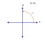
Here, the elements of the Weyl group are considered as orthogonal transformations, acting by matrix multiplication, on the real vector space of roots. One sees that if $- I$ is an element of the Weyl group of a semisimple Lie algebra, then $w 0 = - I$ . In the case of $sl (2, C)$ , the Weyl group is $W = {I, - I}$ .^[75] It follows that each $π μ, μ = 0, 1, \dots$ is equivalent to its dual $π μ *$ . The root system of $sl (2, C) \oplus sl (2, C)$ is shown in the figure to the right.^{[nb 27]} The Weyl group is generated by ${w γ}$ where $w γ$ is reflection in the plane orthogonal to $γ$ as $γ$ ranges over all roots.^{[nb 28]} One sees that $w α \cdotw β = - I$ so $- I \in W$ . Then using the fact that if $π, σ$ are Lie algebra representations and $π \approx σ$ , then $Π \approx Σ$ .^[76] The conclusion for $SO(3; 1) +$ is

\pi _{m,n}^{*}\cong \pi _{m,n},\quad \Pi _{m,n}^{*}\cong \Pi _{m,n},\quad 2m,2n\in \mathbb {N} .

Complex conjugate representations

If $π$ is a representation of a Lie algebra, then $π$ is a representation, where the bar denotes entry-wise complex conjugation in the representative matrices. This follows from that complex conjugation commutes with addition and multiplication.^[77] In general, every irreducible representation $π$ of $sl (n, C)$ can be written uniquely as $π = π + + π -$ , where^[78]

\pi ^{\pm }(X)={\frac {1}{2}}(\pi (X)\pm i\pi (i^{-1}X)),

with $π +$ holomorphic (complex linear) and $π -$ anti-holomorphic (conjugate linear). For $sl (2, C)$ , since $π μ$ is holomorphic, $π μ$ is anti-holomorphic. Direct examination of the explicit expressions for $π μ, 0$ and $π 0, ν$ in equation (S8) below shows that they are holomorphic and anti-holomorphic respectively. Closer examination of the expression (S8) also allows for identification of $π +$ and $π -$ for $π μ, ν$ as $π + μ, ν = π μ \oplus ν + 1$ and $π - μ, ν = π ν \oplus μ + 1$ .

Using the above identities (interpreted as pointwise addition of functions), for $SO(3; 1) +$ yields

{\overline {\pi _{m,n}}}={\overline {\pi _{m,n}^{+}+\pi _{m,n}^{-}}}={\overline {\pi _{m}^{\oplus _{2n+1}}}}+{\overline {{\overline {\pi _{n}}}^{\oplus _{2m+1}}}}=\pi _{n}^{\oplus _{2m+1}}+{\overline {\pi _{m}}}^{\oplus _{2n+1}}=\pi _{n,m}^{+}+\pi _{n,m}^{-}=\pi _{n,m},\quad {\overline {\Pi _{m,n}}}=\Pi _{n,m},\quad 2m,2n\in \mathbb {N} ,

where the statement for the group representations follow from $exp(X)$ = $exp(X)$ . It follows that the irreducible representations $(m, n)$ have real matrix representatives if and only if $m = n$ . Reducible representations on the form $(m, n) \oplus (n, m)$ have real matrices too.

Induced representations

Richard Brauer and wife Ilse 1970. Brauer generalized the spin representations of Lie algebras sitting inside Clifford algebras to spin higher than 1/2. Photo courtesy of MFO.

In general representation theory, if $(π, V)$ is a representation of a Lie algebra g, then there is an associated representation of g on $End V$ , also denoted $π$ , given by

$\pi (X)(A)=[\pi (X),A],\quad A\in \operatorname {End} V,\ X\in {\mathfrak {g}}.$

(I1)

Likewise, a representation $(Π, V)$ of a group $G$ yields a representation $Π$ on $End V$ of $G$ , still denoted $Π$ , given by^[79]

$\Pi (g)(A)=\Pi (g)A\Pi (g)^{-1},\quad A\in \operatorname {End} V,\ g\in G.$

(I2)

Applying this to the Lorentz group, if $(Π, V)$ is a projective representation, then direct calculation using (G4) shows that the induced representation on $End V$ is, in fact, a proper representation, i.e. a representation without phase factors.

In quantum mechanics this means that if $(π, H)$ or $(Π, H)$ is a representation acting on some Hilbert space $H$ , then the corresponding induced representation acts on the set of linear operators on $H$ . As an example, the induced representation of the projective spin $(1 / 2, 0) \oplus (0, 1 / 2)$ representation on $End(H)$ is the non-projective 4-vector (1/2, 1/2) representation.^[30]

For simplicity, consider now only the "discrete part" of $End H$ , that is, given a basis for $H$ , the set of constant matrices of various dimension, including possibly infinite dimensions. A general element of the full $End H$ is the sum of tensor products of a matrix from the simplified $End H$ and an operator from the left out part. The left out part consists of functions of spacetime, differential and integral operators and the like. See Dirac operator for an illustrative example. Also left out are operators corresponding to other degrees of freedom not related to spacetime, such as gauge degrees of freedom in gauge theories.

The induced 4-vector representation of above on this simplified $End H$ has an invariant 4-dimensional subspace that is spanned by the four gamma matrices.^[30] (Note the different metric convention in the linked article.) In a corresponding way, the complete Clifford algebra of spacetime, $Cℓ 3,1 (R)$ , whose complexification is $M 4 (C)$ , generated by the gamma matrices decomposes as a direct sum of representation spaces of a scalar irreducible representation (irrep), the $(0, 0)$ , a pseudoscalar irrep, also the $(0, 0)$ , but with parity inversion eigenvalue −1, see the next section below, the already mentioned vector irrep, $(1 / 2, , 1 / 2)$ , a pseudovector irrep, $(1 / 2, 1 / 2)$ with parity inversion eigenvalue +1 (not −1), and a tensor irrep, $(1, 0) \oplus (0, 1)$ .^[30] The dimensions add up to $1 + 1 + 4 + 4 + 6 = 16$ . In other words,

$Cl_{3,1}(\mathbb {R} )=(0,0)\oplus ({\frac {1}{2}},{\frac {1}{2}})\oplus [(1,0)\oplus (0,1)]\oplus ({\frac {1}{2}},{\frac {1}{2}})_{p}\oplus (0,0)_{p},$

(I3)

where, as is customary, a representation is confused with its representation space. This is, in fact, a reasonably convenient way to show that the algebra spanned by the gammas is 16-dimensional.^[80]

The six-dimensional representation space of the tensor $(1, 0) \oplus (0, 1)$ -representation inside $Cℓ 3,1 (R)$ has two roles. In particular, letting^[81]

$\sigma ^{\mu \nu }=-{\frac {i}{4}}[\gamma ^{\mu },\gamma ^{\nu }],$

(I4)

where ${γ μ \in Cℓ 3,1 (R): μ = 0,1,2,3}$ are the gamma matrices, the ${σ μν \in Cℓ 3,1 (R)}$ , only 6 of which are non-zero due to antisymmetry of the bracket, span the tensor representation space. Moreover, they have the commutation relations of the Lorentz Lie algebra,^[80]

$[\sigma ^{\mu \nu },\sigma ^{\rho \tau }]=i(\eta ^{\tau \mu }\sigma ^{\rho \nu }+\eta ^{\nu \tau }\sigma ^{\mu \rho }-\eta ^{\rho \mu }\sigma ^{\tau \nu }-\eta ^{\nu \rho }\sigma ^{\mu \tau }),$

(I5)

and hence constitute a representation (in addition to being a representation space) sitting inside $Cℓ 3,1 (R)$ , the $(1 / 2, 0) \oplus (0, 1 / 2)$ spin representation. For details, see bispinor and Dirac algebra.

The conclusion is that every element of the complexified $Cℓ 3,1 (R)$ in $End H$ (i.e. every complex 4×4 matrix) has well defined Lorentz transformation properties. In addition, it has a spin-representation of the Lorentz Lie algebra, which upon exponentiation becomes a spin representation of the group, acting on $C 4$ , making it a space of bispinors.

There is also a multitude of other representations that can be said being "induced" by the irreducible ones, such as those obtained in a standard manner by taking direct sums, tensor products, dual representations, quotients, etc. of the irreducible representations. These are not discussed here.

The full Lorentz group

The (possibly projective) $(m, n)$ representation is irreducible as a representation $SO(3; 1) +$ , the identity component of the Lorentz group, in physics terminology the proper orthochronous Lorentz group. If $m = n$ it can be extended to a representation of all of $SO(3; 1)$ , the full Lorentz group, including space parity inversion and time reversal.^[30]

Space parity inversion

For space parity inversion, one considers the adjoint action $Ad P$ of $P \in SO(3; 1)$ on $so (3; 1)$ , where $P$ is the standard representative of space parity inversion, $P = diag(1, -1, -1, -1)$ , given by

$\mathrm {Ad} _{P}(J_{i})=PJ_{i}P^{-1}=J_{i},\qquad \mathrm {Ad} _{P}(K_{i})=PK_{i}P^{-1}=-K_{i}.$

(F1)

It is these properties of $K$ and $J$ under $P$ that motivate the terms vector for $K$ and pseudovector or axial vector for $J$ . In a similar way, if $π$ is any representation of $so (3; 1)$ and $Π$ is its associated group representation, then $Π(SO(3; 1) +)$ acts on the representation of $π$ by the adjoint action, $π(X) \mapsto Π(g) π(X) Π(g) -1$ for $X \in so (3; 1)$ , $g \in SO(3; 1) +$ . If $P$ is to be included in $Π$ , then consistency with (F1) requires that

$\Pi (P)\pi (B_{i})\Pi (P)^{-1}=\pi (A_{i})$

(F2)

holds, where $A$ and $B$ are defined as in the first section. This can hold only if $A i$ and $B i$ have the same dimensions, i.e. only if $m = n$ . When $m \neq n$ then $(m, n) \oplus (n, m)$ can be extended to an irreducible representation of $SO(3; 1) +$ , the orthocronous Lorentz group. The parity reversal representative $Π(P)$ does not come automatically with the general construction of the $(m, n)$ representations. It must be specified separately. The matrix $β = i γ 0$ (or a multiple of modulus −1 times it) may be used in the $(1 / 2, 0) \oplus (0, 1 / 2)$ ^[30] representation.

If parity is included with a minus sign (the $1\times1$ matrix $[-1]$ ) in the $(0,0)$ representation, it is called a pseudoscalar representation.

Time reversal

Time reversal $T = diag(-1, 1, 1, 1)$ , acts similarly on $so (3; 1)$ by^[82]

$\mathrm {Ad} _{T}(J_{i})=TJ_{i}T^{-1}=-J_{i},\qquad \mathrm {Ad} _{T}(K_{i})=TK_{i}T^{-1}=K_{i}.$

(F3)

By explicitly including a representative for $T$ , as well as one for $P$ , one obtains a representation of the full Lorentz group $SO(3; 1)$ . A subtle problem appears however in application to physics, in particular quantum mechanics. When considering the full Poincaré group, four more generators, the $P μ$ , in addition to the $J i$ and $K i$ generate the group. These are interpreted as generators of translations. The time-component $P 0$ is the Hamiltonian $H$ . The operator $T$ satisfies the relation^[83]

$\mathrm {Ad} _{T}(iH)=TiHT^{-1}=-iH$

(F4)

in analogy to the relations above with $so (3; 1)$ replaced by the full Poincaré algebra. By just cancelling the $i$ 's, the result $THT -1 = - H$ would imply that for every state $Ψ$ with positive energy $E$ in a Hilbert space of quantum states with time-reversal invariance, there would be a state $Π(T -1)Ψ$ with negative energy $- E$ . Such states do not exist. The operator $Π(T)$ is therefore chosen antilinear and antiunitary, so that it anticommutes with $i$ , resulting in $THT -1$ = $+ H$ , and its action on Hilbert space likewise becomes antilinear and antiunitary.^[84] It may be expressed as the composition of complex conjugation with multiplication by a unitary matrix.^[85]^[86] This is mathematically sound, see Wigner's theorem, but if one is very strict with terminology, $Π$ is not a representation.

When constructing theories such as QED which is invariant under space parity and time reversal, Dirac spinors may be used, while theories that do not, such as the electroweak force, must be formulated in terms of Weyl spinors. The Dirac representation, (1/2, 0) ⊕ (0, 1/2), is usually taken to include both space parity and time inversions. Without space parity inversion, it is not an irreducible representation.

The third discrete symmetry entering in the CPT theorem along with $P$ and $T$ , charge conjugation symmetry $C$ , has nothing directly to do with Lorentz invariance.^[87]

Infinite-dimensional representations

History

The Lorentz group $SO(3; 1) +$ and its double cover $SL(2, C)$ also have infinite dimensional unitary representations, first studied independently by Bargmann (1947), Gelfand & Naimark (1947) and Harish-Chandra (1947) at the instigation of Paul Dirac. This trail of development begun with Dirac (1936) where he devised matrices $U$ and $B$ necessary for description of higher spin (compare Dirac matrices), elaborated upon by Fierz (1939), see also Fierz & Pauli (1939), and proposed precursors of the Bargmann-Wigner equations. In Dirac (1945) he proposed a concrete infinite-dimensional representation space whose elements were called expansors as a generalization of tensors. These ideas were incorporated by Harish–Chandra and expanded with expinors as an infinite-dimensional generalization of spinors in his 1947 paper.

The Plancherel formula for these groups was first obtained by Gelfand and Naimark through involved calculations. The treatment was subsequently considerably simplified by Harish-Chandra (1951) and Gelfand & Graev (1953), based on an analogue for $SL(2, C)$ of the integration formula of Hermann Weyl for compact Lie groups. Elementary accounts of this approach can be found in Rühl (1970) and Knapp (2001).

The theory of spherical functions for the Lorentz group, required for harmonic analysis on the 3-dimensional unit quasi-sphere in Minkowski space, or equivalently 3-dimensional hyperbolic space, is considerably easier than the general theory. It only involves representations from the spherical principal series and can be treated directly, because in radial coordinates the Laplacian on the hyperboloid is equivalent to the Laplacian on $R$ . This theory is discussed in Takahashi (1963), Helgason (1968), Helgason (2000) and the posthumous text of Jorgenson & Lang (2008).

Action on function spaces

In the classification of the irreducible finite-dimensional representations of above it was never specified precisely how a representative of a group or Lie algebra element acts on vectors in the representation space. The action can be anything as long as it is linear. The point silently adopted was that after a choice of basis in the representation space, everything becomes matrices anyway.

If $V$ is a vector space of functions of a finite number of variables $n$ , then the action on a scalar function $f \in V$ given by

$(\Pi (g)f)(x)=f(\Pi _{x}(g)^{-1}x),\qquad x\in \mathbb {R} ^{n},f\in V$

(H1)

produces another function $Π f \in V$ . Here $Π x$ is an $n$ -dimensional representation, and $Π$ is a possibly infinite-dimensional representation. A special case of this construction is when $V$ is a space of functions defined on the group $G$ itself, viewed as a $n$ -dimensional manifold embedded in $R n$ .^[88] This is the setting in which the Peter–Weyl theorem and the Borel–Weil theorem are formulated. The former demonstrates the existence of a Fourier decomposition of functions on a compact group into characters of finite-dimensional representations.^[29] The completeness of the characters in this sense can thus be used to prove the existence of the highest weight representations.^[89] The latter theorem, providing more explicit representations, makes use of the unitarian trick to yield representations of complex non-compact groups, e.g. $SL(2, C)$ ; in the present case, there is a one-to-one correspondence between representations of $SU(2)$ and holomorphic representations of $SL(2, C)$ . (A group representation is called holomorphic if its corresponding Lie algebra representation is complex linear.) This theorem too can be used to demonstrate the existence of the highest weight representations.^[90]

Euclidean rotations

Main articles: Rotation group SO(3) and Spherical harmonics

The subgroup $SO(3)$ of three-dimensional Euclidean rotations has an infinite-dimensional representation on the Hilbert space $L 2 (S 2) = span{Y ℓ m, ℓ \in N +, - ℓ \leq m \leq ℓ}$ , where the $Y ℓ m$ are spherical harmonics. Its elements are square integrable complex-valued functions^{[nb 29]} on the sphere. The inner product on this space is given by

$\langle f,g\rangle =\int _{\mathbb {S} ^{2}}{\overline {f}}gd\Omega =\int _{0}^{2\pi }\int _{0}^{\pi }{\overline {f}}g\sin \theta d\theta d\varphi .$

(H1)

If $f$ is an arbitrary square integrable function defined on the unit sphere $S 2$ , then it can be expressed as^[91]

$|f\rangle =\sum _{l=1}^{\infty }\sum _{m=-l}^{m=l}|Y_{m}^{l}\rangle \langle Y_{m}^{l}|f\rangle ,\quad f(\theta ,\varphi )=\sum _{l=1}^{\infty }\sum _{m=-l}^{m=l}f_{lm}Y_{m}^{l}(\theta ,\varphi ),$

(H2)

where the expansion coefficients are given by

$f_{lm}=\langle Y_{m}^{l},f\rangle =\int _{\mathbb {S} ^{2}}{\overline {Y_{m}^{l}}}fd\Omega =\int _{0}^{2\pi }\int _{0}^{\pi }{\overline {Y_{m}^{l}}}(\theta ,\varphi )f(\theta ,\varphi )\sin \theta d\theta d\varphi .$

(H3)

The Lorentz group action restricts to that of $SO(3)$ and is expressed as

$(\Pi (R)f)(\theta (x),\varphi (x))=\sum _{l=1}^{\infty }\sum _{m=-l}^{m=l}\sum _{m'=-l}^{m'=l}D_{mm'}^{(l)}(R)f_{lm'}Y_{m}^{l}(\theta (R^{-1}x),\varphi (R^{-1}x)),\qquad R\in \mathrm {SO} (3),\quad x\in \mathbb {S} ^{2}.$

(H4)

This action is unitary, meaning that

$\langle \Pi (R)f,\Pi (R)g\rangle =\langle f,g\rangle \qquad \forall f,g\in \mathbb {S} ^{2},\quad \forall R\in \mathrm {SO} (3).$

(H5)

The $D (ℓ)$ can be obtained from the $D (m, n)$ of above using Clebsch–Gordan decomposition, but they are more easily directly expressed as an exponential of an odd-dimensional $su (2)$ -representation (the 3-dimensional one is exactly $so (3)$ ).^[92]^[93] In this case the space $L 2 (S 2)$ decomposes neatly into an infinite direct sum of irreducible odd finite-dimensional representations $V 2 i + 1, i = 0, 1, \dots$ according to^[94]

$L^{2}(\mathbb {S} ^{2})=\sum _{i=0}^{\infty }V_{2i+1}\equiv \bigoplus _{i=0}^{\infty }\operatorname {span} \{Y_{m}^{2i+1}\}.$

(H6)

This is characteristic of infinite-dimensional unitary representations of $SO(3)$ . If $Π$ is an infinite-dimensional unitary representation on a separable^{[nb 30]} Hilbert space, then it decomposes as a direct sum of finite-dimensional unitary representations.^[91] Such a representation is thus never irreducible. All irreducible finite-dimensional representations $(Π, V)$ can be made unitary by an appropriate choice of inner product,^[91]

\langle f,g\rangle _{U}\equiv \int _{\mathrm {SO} (3)}\langle \Pi (R)f,\Pi (R)g\rangle dg={\frac {1}{8\pi ^{2}}}\int _{0}^{2\pi }\int _{0}^{\pi }\int _{0}^{2\pi }\langle \Pi (R)f,\Pi (R)g\rangle \sin \theta d\varphi d\theta d\psi ,\quad f,g\in V,

where the integral is the unique invariant integral over $SO(3)$ normalized to $1$ , here expressed using the Euler angles parametrization. The inner product inside the integral is any inner product on $V$ .

The Möbius group

Main article: Möbius transformation

The identity component of the Lorentz group is isomorphic to the Möbius group $M$ as is described in detail in Lorentz group. This group can be thought of as conformal mappings of either the complex plane or, via stereographic projection, the Riemann sphere. In this way, the Lorentz group itself can be thought of as acting conformally on the complex plane or on the Riemann sphere. In the plane, a Möbius transformation characterized by the complex numbers $a, b, c, d$ acts on the plane according to

$f(z)={\frac {az+b}{cz+d}},\qquad ad-bc\neq 0$ .

(M1)

and can be represented by complex matrices

$\Pi _{f}={\begin{pmatrix}a&b\\c&d\end{pmatrix}},\qquad \operatorname {det} \Pi _{f}=1.$

(M2)

These are elements of $SL(2, C)$ and are unique up to a sign and $M \approx SL(2, C)/{I, -I} \approx SO(3; 1) +$ . The conformal mappings of the Riemann sphere are thoroughly described in Möbius transformations.

The Riemann P-functions

Main article: Riemann's differential equation

The Riemann P-functions are an example of a set of functions that transform among themselves under the action of the Lorentz (Möbius) group. The Riemann P-functions are expressed as

$w(z)=P\left\{{\begin{matrix}a&b&c&\;\\\alpha &\beta &\gamma &z\\\alpha '&\beta '&\gamma '&\;\end{matrix}}\right\}=\left({\frac {z-a}{z-b}}\right)^{\alpha }\left({\frac {z-c}{z-b}}\right)^{\gamma }P\left\{{\begin{matrix}0&\infty &1&\;\\0&\alpha +\beta +\gamma &0&\;{\frac {(z-a)(c-b)}{(z-b)(c-a)}}\\\alpha '-\alpha &\alpha +\beta '+\gamma &\gamma '-\gamma &\;\end{matrix}}\right\}$ ,

(T1)

where the $a, b, c, α, β, γ, α', β', γ'$ are complex constants. The P-function on the right hand side can be expressed using standard hypergeometric functions giving

$w(z)=\left({\frac {z-a}{z-b}}\right)^{\alpha }\left({\frac {z-c}{z-b}}\right)^{\gamma }\;_{2}F_{1}\left(\alpha +\beta +\gamma ,\alpha +\beta '+\gamma ;1+\alpha -\alpha ';{\frac {(z-a)(c-b)}{(z-b)(c-a)}}\right).$

(T2)

Now define an action of the Lorentz group on the set of all Riemann P-functions by

$u={\frac {Az+B}{Cz+D}}\quad {\text{ and }}\quad \eta ={\frac {Aa+B}{Ca+D}}$

(T3)

and

$\zeta ={\frac {Ab+B}{Cb+D}}\quad {\text{ and }}\quad \theta ={\frac {Ac+B}{Cc+D}},$

(T4)

where $A, B, C, D$ are the entries in

$\pi _{f_{\Lambda }}^{-1}={\begin{pmatrix}A&B\\C&D\end{pmatrix}},$

(T5)

where, $Λ$ is a Lorentz transformation and $f Λ$ is the corresponding Möbius transformation, and, finally, $Π f Λ$ is one of the two possible $SL(2, C)$ matrices corresponding to it, then one has the relation

$P\left\{{\begin{matrix}a&b&c&\;\\\alpha &\beta &\gamma &z\\\alpha '&\beta '&\gamma '&\;\end{matrix}}\right\}=P\left\{{\begin{matrix}\eta &\zeta &\theta &\;\\\alpha &\beta &\gamma &u\\\alpha '&\beta '&\gamma '&\;\end{matrix}}\right\}$

(T6)

expressing the symmetry. The inverse in T5 is needed to obtain a (local) homomorphism.

Principal series

The principal series, or unitary principal series, are the unitary representations induced from the one-dimensional representations of the lower triangular subgroup $B$ of $G = SL(2, C)$ . Since the one-dimensional representations of $B$ correspond to the representations of the diagonal matrices, with non-zero complex entries $z$ and $z -1$ , they thus have the form

\chi _{\nu ,k}{\begin{pmatrix}z&0\\c&z^{-1}\end{pmatrix}}=r^{i\nu }e^{ik\theta },

for $k$ an integer, $ν$ real and with $z = re iθ$ . The representations are irreducible; the only repetitions occur when $k$ is replaced by $- k$ . By definition the representations are realized on L² sections of line bundles on $G / B = S 2$ , which is isomorphic to the Riemann sphere. When $k = 0$ , these representations constitute the so-called spherical principal series.

The restriction of a principal series to the maximal compact subgroup $K = SU(2)$ of $G$ can also be realized as an induced representation of $K$ using the identification $G / B = K / T$ , where $T = B \cap K$ is the maximal torus in $K$ consisting of diagonal matrices with $| z | = 1$ . It is the representation induced from the 1-dimensional representation $z k T$ , and is independent of $ν$ . By Frobenius reciprocity, on $K$ they decompose as a direct sum of the irreducible representations of $K$ with dimensions $| k | + 2 m + 1$ with $m$ a non-negative integer.

Using the identification between the Riemann sphere minus a point and $C$ , the principal series can be defined directly on $L 2 (C)$ by the formula^[95]

\pi _{\nu ,k}{\begin{pmatrix}a&b\\c&d\end{pmatrix}}^{-1}f(z)=|cz+d|^{-2-i\nu }\left({cz+d \over |cz+d|}\right)^{-k}f\left({az+b \over cz+d}\right).

Irreducibility can be checked in a variety of ways:

The representation is already irreducible on $B$ . This can be seen directly, but is also a special case of general results on irreducibility of induced representations due to François Bruhat and George Mackey, relying on the Bruhat decomposition $G = B \cup B s B$ where $s$ is the Weyl group element^[96]

{\begin{pmatrix}0&-1\\1&0\end{pmatrix}}

The action of the Lie algebra ${\mathfrak {g}}$ of $G$ can be computed on the algebraic direct sum of the irreducible subspaces of $K$ can be computed explicitly and the it can be verified directly that the lowest-dimensional subspace generates this direct sum as a ${\mathfrak {g}}$ -module.^[97]^[98]

Complementary series

The for $0 < t < 2$ , the complementary series is defined on $L 2$ functions $f$ on $C$ for the inner product^[99]

(f,g)=\int \int {f(z){\overline {g(w)}}\,dz\,dw \over |z-w|^{2-t}}.

with the action given by^[100]^[101]

\pi _{t}{\begin{pmatrix}a&b\\c&d\end{pmatrix}}^{-1}f(z)=|cz+d|^{-2-t}f\left({az+b \over cz+d}\right).

The complementary series are irreducible and inequivalent. As a representation of $K$ , each is isomorphic to the Hilbert space direct sum of all the odd dimensional irreducible representations of $K = SU(2)$ . Irreducibility can be proved by analyzing the action of ${\mathfrak {g}}$ on the algebraic sum of these subspaces^[97]^[98] or directly without using the Lie algebra.^[102]^[103]

Plancherel theorem

Israïl Moiseevich Gelfand and Mark Naimark found the Plancherel formula for the Lorentz group in 1947.

The only irreducible unitary representations of $SL(2, C)$ are the principal series, the complementary series and the trivial representation. Since $- I$ acts $(-1) k$ on the principal series and trivially on the remainder, these will give all the irreducible unitary representations of the Lorentz group, provided $k$ is taken to be even.

To decompose the left regular representation of $G$ on $L 2 (G)$ , only the principal series are required. This immediately yields the decomposition on the subrepresentations $L 2 (G /\pm I)$ , the left regular representation of the Lorentz group, and $L 2 (G / K)$ , the regular representation on 3-dimensional hyperbolic space. (The former only involves principal series representations with k even and the latter only those with $k = 0$ .)

The left and right regular representation $λ$ and $ρ$ are defined on $L 2 (G)$ by

\lambda (g)f(x)=f(g^{-1}x),\,\,\rho (g)f(x)=f(xg).

Now if $f$ is an element of $C c (G)$ , the operator $π ν, k (f)$ defined by

\pi _{\nu ,k}(f)=\int _{G}f(g)\pi (g)\,dg

is Hilbert–Schmidt. We define a Hilbert space $H$ by

H=\bigoplus _{k\geq 0}HS(L^{2}(C))\otimes L^{2}(R,c_{k}(\nu ^{2}+k^{2})^{1/2}d\nu ),

where

c_{0}=1/4\pi ^{3/2},\,\,c_{k}=1/(2\pi )^{3/2}\,\,(k\neq 0)

and $HS(L 2 (C))$ denotes the Hilbert space of Hilbert–Schmidt operators on $L 2 (C)$ .^{[nb 31]} Then the map $U$ defined on $C c (G)$ by

U(f)(\nu ,k)=\pi _{\nu ,k}(f)

extends to a unitary of $L 2 (G)$ onto $H$ .

The map $U$ satisfies

U(\lambda (x)\rho (y)f)(\nu ,k)=\pi _{\nu ,k}(x)^{-1}\pi _{\nu ,k}(f)\pi _{\nu ,k}(y).

If $f 1$ , $f 2$ are in $C c (G)$ then

(f_{1},f_{2})=\sum _{k\geq 0}c_{k}^{2}\int _{-\infty }^{\infty }{\rm {Tr}}(\pi _{\nu ,k}(f_{1})\pi _{\nu ,k}(f_{2})^{*})(\nu ^{2}+k^{2})\,d\nu .

Thus if $f = f 1 * f 2 *$ denotes the convolution of $f 1$ and $f 2 *$ , and $f_{2}^{*}(g)={\overline {f_{2}(g^{-1})}}$ , then

f(1)=\sum _{k\geq 0}c_{k}^{2}\int _{-\infty }^{\infty }{\rm {Tr}}(\pi _{\nu ,k}(f))(\nu ^{2}+k^{2})\,d\nu .

The last two displayed formulas are usually referred to as the Plancherel formula and the Fourier inversion formula respectively. The Plancherel formula extends to all $f i$ in $L 2 (G)$ . By a theorem of Jacques Dixmier and Paul Malliavin, every function $f$ in $C_{c}^{\infty }(G)$ is a finite sum of convolutions of similar functions, the inversion formula holds for such $f$ . It can be extended to much wider classes of functions satisfying mild differentiability conditions.^[29]

Explicit formulas

Conventions and Lie algebra bases

The metric of choice is given by $η$ = $diag(-1, 1, 1, 1)$ , and the physics convention for Lie algebras and the exponential mapping is used in this article. These choices are arbitrary, but once they are made, fixed. The rationale is to allow the use of a single reference^[30] for several related formulas. One possible choice of basis for the Lie algebra (which is not fixed by the reference) is, in the 4-vector representation, given by

{\begin{aligned}J_{1}&=J^{23}=-J^{32}=i{\biggl (}{\begin{smallmatrix}0&0&0&0\\0&0&0&0\\0&0&0&-1\\0&0&1&0\\\end{smallmatrix}}{\biggr )},\\J_{2}&=J^{31}=-J^{13}=i{\biggl (}{\begin{smallmatrix}0&0&0&0\\0&0&0&1\\0&0&0&0\\0&-1&0&0\\\end{smallmatrix}}{\biggr )},\\J_{3}&=J^{12}=-J^{21}=i{\biggl (}{\begin{smallmatrix}0&0&0&0\\0&0&-1&0\\0&1&0&0\\0&0&0&0\\\end{smallmatrix}}{\biggr )},\\K_{1}&=J^{01}=J^{10}=i{\biggl (}{\begin{smallmatrix}0&1&0&0\\1&0&0&0\\0&0&0&0\\0&0&0&0\\\end{smallmatrix}}{\biggr )},\\K_{2}&=J^{02}=J^{20}=i{\biggl (}{\begin{smallmatrix}0&0&1&0\\0&0&0&0\\1&0&0&0\\0&0&0&0\\\end{smallmatrix}}{\biggr )},\\K_{3}&=J^{03}=J^{30}=i{\biggl (}{\begin{smallmatrix}0&0&0&1\\0&0&0&0\\0&0&0&0\\1&0&0&0\\\end{smallmatrix}}{\biggr )}.\end{aligned}}

The commutation relations of the Lie algebra so(3; 1) are^[30]

[J^{\mu \nu },J^{\rho \sigma }]=i(\eta ^{\sigma \mu }J^{\rho \nu }+\eta ^{\nu \sigma }J^{\mu \rho }-\eta ^{\rho \mu }J^{\sigma \nu }-\eta ^{\nu \rho }J^{\mu \sigma }).

In three-dimensional notation, these are^[30]

[J_{i},J_{j}]=i\epsilon _{ijk}J_{k},\quad [J_{i},K_{j}]=i\epsilon _{ijk}K_{k},\quad [K_{i},K_{j}]=-i\epsilon _{ijk}J_{k}.

The choice of basis above satisfies the relations, but other choices are possible. The multiple use of the symbol $J$ above and in the sequel should be observed.

Let $π (m, n) : so (3; 1) \to gl (V)$ , where $V$ is a vector space, denote the irreducible representations of $so (3; 1)$ according to the $(m, n)$ classification. In components, with $- m \leq a, a' \leq m$ , $- n \leq b, b' \leq n$ , the representations are given by^[30]

{\begin{aligned}(\pi _{m,n}(J_{i}))_{a'b',ab}&=\delta _{b'b}(J_{i}^{(m)})_{a'a}+\delta _{a'a}(J_{i}^{(n)})_{b'b},\\(\pi _{m,n}(K_{i}))_{a'b',ab}&=i(\delta _{a'a}(J_{i}^{(n)})_{b'b}-\delta _{b'b}(J_{i}^{(m)})_{a'a}),\end{aligned}}

where $δ$ is the Kronecker delta and the $J i (n)$ are the $(2 n + 1)$ -dimensional irreducible representations of $so (3)$ , also termed spin matrices or angular momentum matrices. These are also explicitly given in ^[30]

{\begin{aligned}(J_{3}^{(j)})_{a'a}&=a\delta _{a'a},\\(J_{1}^{(j)}\pm iJ_{2}^{(j)})_{a'a}&={\sqrt {(j\mp a)(j\pm a+1)}}\delta _{a',a\pm 1}.\end{aligned}}

Weyl spinors and bispinors

P.A.M Dirac put the

(1 / 2, 0) \oplus (0, 1 / 2)

-representation to use in the Dirac equation.

By taking, in turn, $m = 1 / 2$ , $n = 0$ and $m = 0$ , $n = 1 / 2$ and by setting

J_{i}^{({\frac {1}{2}})}={\frac {1}{2}}\sigma _{i}

in the general expression (G1), and by using the trivial relations 1₁ = 1 and $J (0) = 0$ , one obtains

${\begin{aligned}\pi _{({\frac {1}{2}},0)}(J_{i})&={\frac {1}{2}}(\sigma _{i}\otimes 1_{(1)}+1_{(2)}\otimes J_{i}^{(0)})={\frac {1}{2}}\sigma _{i}\quad \pi _{({\frac {1}{2}},0)}(K_{i})={\frac {i}{2}}(1_{(2)}\otimes J_{i}^{(0)}-\sigma _{i}\otimes 1_{(1)})=-{\frac {i}{2}}\sigma _{i},\\\pi _{(0,{\frac {1}{2}})}(J_{i})&={\frac {1}{2}}(J_{i}^{(0)}\otimes 1_{(2)}+1_{(1)}\otimes \sigma _{i})={\frac {1}{2}}\sigma _{i}\quad \pi _{(0,{\frac {1}{2}})}(K_{i})={\frac {i}{2}}(1_{(1)}\otimes \sigma _{i}-J_{i}^{(0)}\otimes 1_{(2)})=+{\frac {i}{2}}\sigma _{i}.\end{aligned}}$

(W1)

These are the left-handed and right-handed Weyl spinor representations. They act by matrix multiplication on 2-dimensional complex vector spaces (with a choice of basis) $V L$ and $V R$ , whose elements $Ψ L$ and $Ψ R$ are called left- and right-handed Weyl spinors respectively. Given $(π (1 / 2,0), V L)$ and $(π (0, 1 / 2), V R)$ one may form their direct sum as representations,^[104]

${\begin{aligned}\pi _{({\frac {1}{2}},0)\oplus (0,{\frac {1}{2}})}(J_{i})&={\frac {1}{2}}{\biggl (}{\begin{matrix}\sigma _{i}&0\\0&\sigma _{i}\\\end{matrix}}{\biggr )},\\\pi _{({\frac {1}{2}},0)\oplus (0,{\frac {1}{2}})}(K_{i})&={\frac {i}{2}}{\biggl (}{\begin{matrix}\sigma _{i}&0\\0&-\sigma _{i}\\\end{matrix}}{\biggr )}\\\end{aligned}}.$

(D1)

This is, up to a similarity transformation, the $(1 / 2,0) \oplus (0, 1 / 2)$ Dirac spinor representation of $so (3; 1)$ . It acts on the 4-component elements $(Ψ L, Ψ R)$ of $(V L \oplus V R)$ , called bispinors, by matrix multiplication. The representation may be obtained in a more general and basis independent way using Clifford algebras. These expressions for bispinors and Weyl spinors all extend by linearity of Lie algebras and representations to all of $so (3; 1)$ . Expressions for the group representations are obtained by exponentiation.

Remarks

↑ The way in which it enters may take many shapes depending on the theory at hand. While not being the present topic, some details will be provided in footnotes like this one.
↑ Weinberg 2002, p. 1 "If it turned out that a system could not be described by a quantum field theory, it would be a sensation; if it turned out it did not obey the rules of quantum mechanics and relativity, it would be a cataclysm."
↑ While the electromagnetic field together with the gravitational field are the only classical fields providing accurate descriptions of nature, other types of classical fields are important too. In the approach to QFT referred to as second quantization, one begins with one or more classical fields, where e.g. the wave functions solving the Dirac equation are considered as classical fields prior to quantization. While second quantization and the Lagrangian formalism associated with it is not a fundamental aspect of QFT, it is the case that so far all quantum field theories can be approached this was, including the standard model. It these cases, there are classical versions of the field equations following from the Euler–Lagrange equations derived from the Lagrangian using the principle of least action. These field equations must be relativistically invariant, and their solutions must transform under some representation of the Lorentz group.
The action of the Lorentz group on the space of field configurations (a field configuration is the spacetime history of a particular solution, e.g the electromagnetic field in all of space over all time is one field configuration) resemble the action on the Hilbert spaces of quantum mechanics, except that the commutator brackets are replaced by field theoretical Poisson bracket..
For a short introduction to classical field theory from this point of view, see Greiner & Reinhardt (1996, Chapter 2).
↑ The most useful relativistic quantum mechanics one-particle theories (there are no fully consistent such theories) are the Klein–Gordon equation and the Dirac equation in their original setting. They are relativistically invariant and their solutions transform under the Lorentz group as Lorentz scalars and bispinors respectively.
See Greiner & Müller (1994) for an extensive treatment of these equations.
↑ In QFT, the demand for relativistic invariance enters, among other ways in that the S-matrix necessarily must be Lorentz invariant. This has the implication that there is one or more infinite-dimensional representation of the Lorentz group acting on Fock space. One way to guarantee the existence of such representations is the existence of a Lagrangian description of the system using the canonical formalism.
See Weinberg (2003) for a treatment from a very general point of view.
↑ In theories in which spacetime can have more than $D = 4$ dimensions, the generalized Lorentz groups $O(D - 1; 1)$ of the appropriate dimension enter. For their representation theory, see Bekaert & Boulanger (2006).
The requirement of Lorentz invariance takes on perhaps its most dramatic effect in string theory. Classical relativistic strings can be handled in the Lagrangian framework by using the Nambu–Goto action. This results in a relativistically invariant theory in any spacetime dimension. But as it turns out, the theory of open and closed bosonic strings (the simplest string theory) is impossible to quantize in such a way that the Lorentz group is represented on the space of states (a Hilbert space) unless the dimension of spacetime is 26!
See Zwiebach (2004) for this topic.
The corresponding result for superstring theory, deduced again by demanding Lorentz invariance, but now with supersymmetry (now the Poincaré algebra is replaced by the Super-Poincaré algebra) is that the dimension of spacetime must be 10.
↑ By "beyond" is here meant superstring theory, M-theory and more. For instance, string theory really is a theory of one string (though it can represent many different particles depending on its state). String field theory would be the equivalent of ordinary quantum field theory.
↑ At the level of quantum fields in QFT similar results hold. For instance, there are versions (free field equations, i.e. without interaction terms) of the Klein–Gordon equation, the Dirac equation, the Maxwell equations, the Proca equation, the Rarita–Schwinger equation, and the Einstein field equations that can systematically be deduced by starting from a given representation of the Lorentz group. In general, these are collectively the quantum field theory versions of the Bargmann–Wigner equations.
See Weinberg 2002, Chapter 5 for deduction of some of these.
↑ In 1945 Harish-Chandra came to see Dirac in Cambridge. He became convinced that he was not suitable for theoretical physics. Harish-Chandra had found an error in a proof by Dirac in his work on the Lorentz group. Dirac said "I am not interested in proofs but only interested in what nature does."
Harish-Chandra later wrote "This remark confirmed my growing conviction that I did not have the mysterious sixth sense which one needs in order to succeed in physics and I soon decided to move over to mathematics." Dirac did however suggest the topic of his thesis, the classification of the irreducible infinite-dimensional representations of the Lorentz group.
See Dalitz & Peierls 1986
↑ Knapp 2001 The rather mysterious looking third isomorphism is proved in chapter 2, paragraph 4.
↑ Tensor products of representations, $π g \otimes π h$ of $g \oplus h$ can, when both factors come from the same Lie algebra $(h = g)$ , either be thought of as a representation of $g$ or $g \oplus g$ .
↑ The "traceless" property can be expressed as $S αβ g αβ = 0$ , or $S α α = 0$ , or $S αβ g αβ = 0$ depending on the presentation of the field: covariant, mixed, and contravariant respectively.
↑ This is provided parity is a symmetry. Else there would be two flavors, (3/2, 0) and (0, 3/2) in analogy with neutrinos.
↑ It's a rather deep fact that all finite-dimensional Lie algebras are linear. See Ado's theorem. The corresponding statement for compact Lie groups is true, but not for general Lie groups.
↑ Hall 2003, Equation 2.16. Due to the physicist conventions, the formula here differs with a factor of $i$ in the exponent.
↑ In particular, $A$ commutes with the Pauli matrices, hence with all of $SU(2)$ making Schur's lemma applicable.
↑ The kernel of a Lie algebra homomorphism is an ideal, hence a subspace. Since $p$ is $2:1$ and both $SL(2, C)$ and $SO(3; 1) +$ are $6$ -dimensional, the kernel must be $0$ -dimensional, hence ${\emptyset}$ .
↑ The exponential map is one-to-one in a neighborhood of the identity in $SL(2, C)$ , hence the composition $exp \circ σ \circ log:SL(2, C) \to SO(3; 1) +$ , where $σ$ is the Lie algebra isomorphism, is onto an open neighborhood $U \subset SO(3; 1) +$ containing the identity. Such a neighborhood generates the connected component.
↑ Rossmann 2002 From Section 2.1 Example 4: This can be seen as follows. The matrix q has eigenvalues ${-1, -1}$ , but it is not diagonalizable. If $q = exp(Q)$ , then $Q$ has eigenvalues $λ, -λ$ with $λ = iπ + 2π ik$ for some $k$ because the tracelessness of $sl (2, C)$ -matrices forces them to be negatives of each other. But then $Q$ is diagonalizable, hence $q$ is diagonalizable. This is a contradiction.
↑ Rossmann 2002 Proposition 10, paragraph 6.3. This is a consequence of the Peter-Weyl theorem.
↑ Hall 2003 Any discrete normal subgroup of a path connected group $G$ is contained in the center $Z$ of $G$ . See Exercise 11, Chapter 1.
↑ A semisimple Lie group does not have any non-discrete normal abelian subgroups. This can be taken as the definition of semisimplicity.
↑ A simple group does not have any non-discrete normal subgroups.
↑ Lee 2003 Lemma A.17 (c). Closed subsets of compact sets are compact.
↑ Lee 2003 Lemma A.17 (a). If $f : X \to Y$ is continuous, $X$ is compact, then $f (X)$ is compact.
↑ This is one of the conclusions of Cartan's theorem, the theorem of the highest weight. See Hall (2003) Chapter 6.
↑ Hall 2003 The root system is the union of two copies of $A 1$ , where each copy resides in its own dimensions in the embedding vector space.
↑ Rossmann 2003 This definition is equivalent to the definition in terms of the connected Lie group whose Lie algebra is the Lie algebra of the root system under consideration.
↑ The elements of $L 2 (S 2)$ are actually equivalence classes of functions. two functions are declared equivalent if they differ merely on a set of measure zero. The integral is the Lebesgue integral in order to obtain a complete inner product space.
↑ A Hilbert space is separable if and only if it has a countable basis. All separable Hilbert spaces are isomorphic.
↑ Note that for a Hilbert space $H$ , $HS(H)$ may be identified canonically with the Hilbert space tensor product of $H$ and its conjugate space.

Notes

1 2 Greiner 1996
↑ Misner, Thorne & Wheeler 1973
↑ Bargmann & Wigner 1948
↑ Bekaert & Boulanger 2006
↑ These facts can be found in most elementary mathematics texts, and many physics texts. See e.g. Rossmann (2002), Hall (2003)
↑ See e.g. Hall (2003)
1 2 3 Wigner 1939
↑ Hall 2003 Appendix D2.
↑ Weinberg 2003
↑ Lie 1888, 1890, 1893
↑ Killing 1888
↑ Cartan 1913
↑ Brauer & Weyl 1935 Spinors in n dimensions.
↑ Weyl 1931 The Theory of Groups and Quantum Mechanics.
↑ Weyl 1939 The Classical Groups. Their Invariants and Representations.
↑ Harish-Chandra 1947 Infinite irreducible representations of the Lorentz group.
↑ Wigner 1939 On unitary representations of the inhomogeneous Lorentz group.
↑ Bargmann 1947 Irreducible unitary representations of the Lorenz group.
↑ Bargmann was also a mathematician. He worked as Albert Einsteins assistant at the Institute for Advanced Study in Princeton.
↑ Bargmann & Wigner 1948 Group theoretical discussion of relativistic wave equations.
↑ Dirac 1928
↑ Weinberg 2003 Equation 5.6.7-8
↑ Weinberg 2003, Chapter 5
↑ Weinberg 2003 Equation 5.6.9-11
1 2 3 4 Hall 2003, Chapter 6
↑ Hall 2003, Chapter 4
↑ Rossmann 2002 Section 6.5
1 2 Knapp 2001 See section 2.3
1 2 3 4 5 6 7 8 Knapp 2001
1 2 3 4 5 6 7 8 9 10 11 12 13 14 Weinberg 2002, Chapter 5
↑ Weinberg 2003 See footnote on p. 232.
↑ Lie 1888
↑ Rossmann 2002, Section 2.5
↑ Rossmann 2002 Theorem 1, Paragraph 2.5.
1 2 Rossmann 2002 Proposition 3, Paragraph 2.5.
↑ Rossmann 2002 Theorem 1, Paragraph 2.6.
1 2 3 4 5 Hall 2003, Theorem 2.27, Chapter 2.
↑ Hall 2003 Section 3.1.
↑ Hall 2003 Formulae 3.1, 3.2 and 3.3 modified for physics convention.
↑ Hall 2003 See section 3.6 for a detailed account.
↑ Hall 2003 Exercise 10 Chapter 3.
↑ Rossmann 2002
↑ Hall 2003 Step 5 in proof of theorem 3.7
↑ Weinberg 2002, Appendix B, Chapter 2
↑ Weinberg 2002, Section 2.7, Chapter 2
↑ Wigner 1939, p.27
↑ Weinberg 2003, Section 2.7
↑ Gelfand, Minlos & Shapiro 1963 This construction of the covering group is treated in paragraph 4, section 1, chapter 1 in Part II.
1 2 Hall 2003 Chapter 4.
1 2 Knapp 2001 Chapter 2.
↑ Knapp 2001 Equation 2.1.
↑ Hall 2003 Equation 4.2.
↑ Hall 2003 Equation after 4.2.
↑ Hall 2003 Equation 4.3.
↑ Hall 2003 Equation after 4.3
↑ Knapp 2001 Equation 2.4.
↑ Rossmann 2002 Section 2.1
↑ Rossmann 2002 Section 2.1 Example 4.
↑ Hall 2003 Corollary 2.31.
↑ Hall 2003 Appendix A.
↑ Weinberg 2003 Chapter 5.
↑ Hall 2003 Theorem 7.15.
↑ Hall 2003 Theorem 7.43.
↑ Hall 2003 p. 235.
↑ Rossmann 2002 Propositions 3 and 6 paragraph 2.5.
↑ Hall 2003 See exercise 1, Chapter 6.
↑ Bekaert & Boulanger 2006 p.4.
↑ Hall 2003 Proposition 1.20.
↑ Lee 2003 Theorem 8.30
↑ Weinberg 2002Chapters 2, 5.
↑ Weinberg 2002 This is outlined (very briefly) on page 232, hardly more than a footnote.
↑ Hall 2003 Proposition 7.39.
↑ Hall 2003 Theorem 7.40.
↑ Hall 2003 Theorem 7.40.
↑ Hall 2003 See section 6.6 for a detailed discussion.
↑ Hall 2003 Second item in proposition 4.5.
↑ Hall 2003 p.219
↑ Rossmann 2002 See exercise 3 in paragraph 6.5.
↑ Hall 2003 See appendix D.3
1 2 Weinberg 2002 Section 5.4.
↑ Weinberg 2002 Eqn 5.4.6
↑ Weinberg 2003 Equation 2.6.5.
↑ Weinberg 2003 Equation following 2.6.6.
↑ Weinberg 2002 Chapter 2.
↑ Greiner, W (2000), Relativistic Quantum Mechanics, ISBN 3-540-67457-8
↑ For a detailed discussion of the spin 0, 1/2 and 1 cases, see Greiner & Reinhardt 1996.
↑ Weinberg 2002, Chapter 3
↑ Rossmann 2002 See section 6.1 for more examples, both finite-dimensional and infinite-dimensional.
↑ Hall 2003, Chapter 7
↑ Hall 2003, Chapter 7
1 2 3 Gelfand, Minlos & Shapiro 1963
↑ In Quantum Mechanics - non-relativistic theory by Landau and Lifshitz the lowest order $D$ are calculated analytically.
↑ Curtright, Fairlie & Zachos 2014 A formula for $D (ℓ)$ valid for all ℓ is given.
↑ Hall 2003 Section 4.3.5.
↑ Gelfand & Graev 1969
↑ Knapp 2001, Chapter II
1 2 Harish-Chandra 1947
1 2 Taylor 1986
↑ Knapp 2001 Chapter 2. Equation 2.12.
↑ Bargmann 1947
↑ Gelfand & Gaev 1963
↑ Gelfand & Naimark 1947
↑ Takahashi 1963, p. 343
↑ Weinberg 2002, Equations (5.4.19) and (5.4.20)

Freely available online references

Bekaert, X.; Boulanger, N. (2006). "The unitary representations of the Poincare group in any spacetime dimension". arXiv:hep-th/0611263. Expanded version of the lectures presented at the second Modave summer school in mathematical physics (Belgium, August 2006).
Curtright, T L; Fairlie, D B; Zachos, C K (2014), "A compact formula for rotations as spin matrix polynomials", SIGMA, 10: 084, arXiv:1402.3541, Bibcode:2014SIGMA..10..084C, doi:10.3842/SIGMA.2014.084 Group elements of SU(2) are expressed in closed form as finite polynomials of the Lie algebra generators, for all definite spin representations of the rotation group.

References

Bargmann, V. (1947), "Irreducible unitary representations of the Lorenz group", Ann. of Math., 48 (3): 568–640, doi:10.2307/1969129, JSTOR 1969129 (the representation theory of SO(2,1) and SL(2, R); the second part on SO(3; 1) and SL(2, C), described in the introduction, was never published).
Bargmann, V.; Wigner, E. P. (1948), "Group theoretical discussion of relativistic wave equations", Proc. Natl. Acad. Sci. USA, 34 (5): 211–23, Bibcode:1948PNAS...34..211B, doi:10.1073/pnas.34.5.211
Brauer, R.; Weyl, H. (1935), "Spinors in n dimensions", Amer. J. Math., 57 (2): 425–449, doi:10.2307/2371218
Cartan, Élie (1913), "Les groupes projectifs qui ne laissant invariante aucun multiplicité plane", Bull. Soc. Math. (in French), 41: 53–96
Dalitz, R. H.; Peierls, Rudolf (1986). "Paul Adrien Maurice Dirac. 8 August 1902-20 October 1984". Biogr. Mems Fell. R. Soc. 32: 138–185. doi:10.1098/rsbm.1986.0006.
Dirac, P. A. M. (1928), "The Quantum Theory of the Electron", Proc. Roy. Soc. A, 117 (778): 610, Bibcode:1928RSPSA.117..610D, doi:10.1098/rspa.1928.0023 (free access)
Dirac, P. A. M. (1936), Relativistic wave equations, 155 (886), Proc. Roy. Soc. A, pp. 447–459, Bibcode:1936RSPSA.155..447D, doi:10.1098/rspa.1936.0111
Dirac, P. A. M. (1945), Unitary representations of the Lorentz group, 183 (994), Proc. Roy. Soc. A, pp. 284–295, Bibcode:1945RSPSA.183..284D, doi:10.1098/rspa.1945.0003
Dixmier, J.; Malliavin, P. (1978), "Factorisations de fonctions et de vecteurs indéfiniment différentiables", Bull. Sc. Math. (in French), 102: 305–330
Fierz, M. (1939), "Über die relativistische theorie Kräftefreier teilchen mit beliebigem spin", Helv. Phys. Acta (in German), 12 (1): 3–37, doi:10.5169/seals-110930(pdf download available)
Fierz, M.; Pauli, W. (1939), "On relativistic wave equations for particles of arbitrary spin in an electromagnetic field", Proc.Roy. Soc. A, 173 (953): 211–232, Bibcode:1939RSPSA.173..211F, doi:10.1098/rspa.1939.0140
Gelfand, I. M.; Graev, M. I. (1953), "On a general method of decomposition of the regular representation of a Lie group into irreducible representations", Doklady Akademii Nauk SSSR, 92: 221–224
Gelfand, I. M.; Graev, M. I.; Pyatetskii-Shapiro, I. I. (1969), Representation theory and automorphic functions, Academic Press, ISBN 0-12-279506-7
Gelfand, I.M.; Minlos, R.A.; Shapiro, Z. Ya. (1963), Representations of the Rotation and Lorentz Groups and their Applications, New York: Pergamon Press
Gelfand, I. M.; Naimark, M. A. (1947), "Unitary representations of the Lorentz group" (PDF), Izvestiya Akad. Nauk SSSR. Ser. Mat. (in Russian), 11 (5): 411–504, retrieved 2014-12-15(Pdf from Math.net.ru)
Greiner, W.; Müller, B. (1994). Quantum Mechanics: Symmetries (2nd ed.). Springer. ISBN 978-3540580805.
Greiner, W.; Reinhardt, J. (1996), Field Quantization, Springer, ISBN 3-540-59179-6
Harish-Chandra (1947), "Infinite irreducible representations of the Lorentz group", Proc. Roy. Soc. A, 189 (1018): 372–401, Bibcode:1947RSPSA.189..372H, doi:10.1098/rspa.1947.0047
Harish-Chandra (1951), "Plancherel formula for complex semi-simple Lie groups", Proc. Natl. Acad. Sci. U.S.A., 37 (12): 813–818, Bibcode:1951PNAS...37..813H, doi:10.1073/pnas.37.12.813
Hall, Brian C. (2003), Lie Groups, Lie Algebras, and Representations An Elementary Introduction, Springer, ISBN 0-387-40122-9
Helgason, S. (1968), Lie groups and symmetric spaces, Battelle Rencontres, Benjamin, pp. 1–71 (a general introduction for physicists)
Helgason, S. (2000), Groups and geometric analysis. Integral geometry, invariant differential operators, and spherical functions (corrected reprint of the 1984 original), Mathematical Surveys and Monographs, 83, American Mathematical Society, ISBN 0-8218-2673-5
Jorgenson, J.; Lang, S. (2008), The heat kernel and theta inversion on SL(2,C), Springer Monographs in Mathematics, Springer, ISBN 978-0-387-38031-5
Killing, Wilhelm (1888), "Die Zusammensetzung der stetigen/endlichen Transformationsgruppen", Mathematische Annalen (in German), 31 (2 (June)): 252–290, doi:10.1007/bf01211904
Knapp, Anthony W. (2001), Representation theory of semisimple groups. An overview based on examples., Princeton Landmarks in Mathematics, Princeton University Press, ISBN 0-691-09089-0 (elementary treatment for SL(2,C))
Lee, J. M. (2003), Introduction to Smooth manifolds, Springer Graduate Texts in Mathematics, 218, ISBN 0-387-95448-1
Lie, Sophus (1888), Theorie der Transformationsgruppen I(1888), II(1890), III(1893) (in German)
Misner, Charles W.; Thorne, Kip. S.; Wheeler, John A. (1973), Gravitation, W. H. Freeman, ISBN 0-7167-0344-0
Naimark, M.A. (1964), Linear representations of the Lorentz group (translated from the Russian original by Ann Swinfen and O. J. Marstrand), Macmillan
Rossmann, Wulf (2002), Lie Groups - An Introduction Through Linear Groups, Oxford Graduate Texts in Mathematics, Oxford Science Publications, ISBN 0 19 859683 9
Rühl, W. (1970), The Lorentz group and harmonic analysis, Benjamin (a detailed account for physicists)
Takahashi, R. (1963), "Sur les représentations unitaires des groupes de Lorentz généralisés", Bull. Soc. Math. France (in French), 91: 289–433
Taylor, M. E. (1986), Noncommutative harmonic analysis, Mathematical Surveys and Monographs, 22, American Mathematical Society, ISBN 0-8218-1523-7 , Chapter 9, SL(2, C) and more general Lorentz groups
Weinberg, S. (2002), The Quantum Theory of Fields, 1, Cambridge University Press, ISBN 0-521-55001-7
Weyl, H. (1939), The Classical Groups. Their Invariants and Representations, Princeton University Press, ISBN 978-0-691-05756-9, MR 0000255
Weyl, H. (1931), The Theory of Groups and Quantum Mechanics, Dover, ISBN 0-486-60269-9
Wigner, E. P. (1939), "On unitary representations of the inhomogeneous Lorentz group", Annals of Mathematics, 40 (1): 149 204, Bibcode:1939AnMat..40..922E, doi:10.2307/1968551, MR 1503456 .
Zwiebach, B. (2004). A First Course in String Theory. Cambridge University Press. ISBN 0 521 83143 1.

This article is issued from Wikipedia - version of the 12/3/2016. The text is available under the Creative Commons Attribution/Share Alike but additional terms may apply for the media files.

Representation theory of the Lorentz group

Finite-dimensional representations

History

The Lie algebra

The unitarian trick

The representations

sl(2, C)

so(3; 1)

Common representations

The group

The Lie correspondence

Lie algebra representations from group representations

Group representations from Lie algebra representations

Local existence and uniqueness

Global existence and uniqueness

Partition independence

Path independence

Global homomorphism

Surjectiveness of exponential mapping

Consistency

Projective representations

The covering group

A geometric view

An algebraic view

Representations of SL(2, C) and sl(2, C)

Concrete realization

Non-surjectiveness of exponential mapping

SO(3; 1)+-representations from SL(2, C)-representations

SL(2, C)-representations from SO(3; 1)+-representations

Properties of the (m, n) representations

Faithfulness

Non-unitarity

Restriction to SO(3)

Spinors

Dual representations

Complex conjugate representations

Induced representations

The full Lorentz group

Space parity inversion

Time reversal

Infinite-dimensional representations

History

Action on function spaces

Euclidean rotations

The Möbius group

The Riemann P-functions

Principal series

Complementary series

Plancherel theorem

Explicit formulas

Conventions and Lie algebra bases

Weyl spinors and bispinors

See also

Remarks

Notes

Freely available online references

References

Representations of $SL(2, C)$ and $sl(2, C)$

$SO(3; 1) +$ -representations from $SL(2, C)$ -representations

$SL(2, C)$ -representations from $SO(3; 1) +$ -representations