Level set method

Video of spiral being propagated by level sets (mean curvature flow) in 2D. LHS shows zero-level solution. RHS shows the level-set scalar field.

Level set methods (LSM) are a conceptual framework for using level sets as a tool for numerical analysis of surfaces and shapes. The advantage of the level set model is that one can perform numerical computations involving curves and surfaces on a fixed Cartesian grid without having to parameterize these objects (this is called the Eulerian approach).^[1] Also, the level set method makes it very easy to follow shapes that change topology, for example when a shape splits in two, develops holes, or the reverse of these operations. All these make the level set method a great tool for modeling time-varying objects, like inflation of an airbag, or a drop of oil floating in water.

An illustration of the level set method

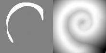
The figure on the right illustrates several important ideas about the level set method. In the upper-left corner we see a shape; that is, a bounded region with a well-behaved boundary. Below it, the red surface is the graph of a level set function $\varphi$ determining this shape, and the flat blue region represents the xy-plane. The boundary of the shape is then the zero level set of $\varphi$ , while the shape itself is the set of points in the plane for which $\varphi$ is positive (interior of the shape) or zero (at the boundary).

In the top row we see the shape changing its topology by splitting in two. It would be quite hard to describe this transformation numerically by parameterizing the boundary of the shape and following its evolution. One would need an algorithm able to detect the moment the shape splits in two, and then construct parameterizations for the two newly obtained curves. On the other hand, if we look at the bottom row, we see that the level set function merely translated downward. This is an example of when it can be much easier to work with a shape through its level set function than with the shape directly, where using the shape directly would need to consider and handle all the possible deformations the shape might undergo.

Thus, in two dimensions, the level set method amounts to representing a closed curve $\Gamma$ (such as the shape boundary in our example) using an auxiliary function $\varphi$ , called the level set function. $\Gamma$ is represented as the zero level set of $\varphi$ by

\Gamma = \{(x, y)|\, \varphi(x, y) = 0 \}, \,

and the level set method manipulates $\Gamma$ implicitly, through the function $\varphi$ . This function $\varphi$ is assumed to take positive values inside the region delimited by the curve $\Gamma$ and negative values outside.^[2]^[3]

The Level Set Equation

If the curve $\Gamma$ moves in the normal direction with a speed $v$ , then the level set function $\varphi$ satisfies the level set equation

\frac{\partial\varphi}{\partial t} = v|\nabla \varphi|

Here, $|\cdot |$ is the Euclidean norm (denoted customarily by single bars in PDEs), and $t$ is time. This is a partial differential equation, in particular a Hamilton–Jacobi equation, and can be solved numerically, for example by using finite differences on a Cartesian grid.^[2]^[3]

The numerical solution of the level set equation, however, requires sophisticated techniques. Simple finite difference methods fail quickly. Upwinding methods, such as the Godunov method, fare better; however the level set method does not guarantee the conservation of the volume and the shape of the level set in an advection field that does conserve the shape and size, for example uniform or rotational velocity field. Instead, the shape of the level set may get severely distorted and the level set may vanish over several time steps. For this reason, high-order finite difference schemes are generally required, such as high-order essentially non-oscillatory (ENO) schemes, and even then, the feasibility of long-time simulations is questionable. Further sophisticated methods to deal with this difficulty have been developed, e.g., combinations of the level set method with tracing marker particles advected by the velocity field.^[4]

Example

Consider a unit circle in $\mathbf{R}^2$ , shrinking in on itself at a constant rate, i.e. each point on the boundary of the circle moves along its inwards pointing normal at some fixed speed. The circle will shrink, and eventually collapse down to a point. If an initial distance field is constructed (i.e. a function whose value is the signed euclidean distance to the boundary (positive interior, negative exterior)) on the initial circle, the normalised gradient of this field will be the circle normal.

If the field has a constant value subtracted from it in time, the zero level (which was the initial boundary) of the new fields will also be circular, and will similarly collapse to a point. This is due to this being effectively the temporal integration of the Eikonal equation with a fixed front velocity.

History

The level set method was developed in the 1980s by the American mathematicians Stanley Osher and James Sethian. It has become popular in many disciplines, such as image processing, computer graphics, computational geometry, optimization, and computational fluid dynamics.

A number of level set data structures have been developed to facilitate the use of the level set method in computer applications.

Applications

- Computational Fluid Dynamics - Trajectory Planning - Optimization - Image Processing

References

↑ Osher, S.; Sethian, J. A. (1988), "Fronts propagating with curvature-dependent speed: Algorithms based on Hamilton–Jacobi formulations" (PDF), J. Comput. Phys., 79: 12–49., Bibcode:1988JCoPh..79...12O, doi:10.1016/0021-9991(88)90002-2
1 2 Osher, Stanley J.; Fedkiw, Ronald P. (2002). Level Set Methods and Dynamic Implicit Surfaces. Springer-Verlag. ISBN 0-387-95482-1.
1 2 Sethian, James A. (1999). Level Set Methods and Fast Marching Methods : Evolving Interfaces in Computational Geometry, Fluid Mechanics, Computer Vision, and Materials Science. Cambridge University Press. ISBN 0-521-64557-3.
↑ Enright, D.; Fedkiw, R. P.; Ferziger, J. H.; Mitchell, I. (2002), "A hybrid particle level set method for improved interface capturing" (PDF), J. Comput. Phys., 183: 83–116., Bibcode:2002JCoPh.183...83E, doi:10.1006/jcph.2002.7166

External links

See Ronald Fedkiw's academic web page for many stunning pictures and animations showing how the level set method can be used to model real life phenomena, like fire, water, cloth, fracturing materials, etc.
Multivac is a C++ library for front tracking in 2D with level set methods.
James Sethian's web page on level set method.
Stanley Osher's homepage.

Numerical partial differential equations by method

Finite difference

Parabolic	Forward-time central-space (FTCS) Crank–Nicolson

Hyperbolic	Lax–Friedrichs Lax–Wendroff MacCormack Upwind Method of characteristics

Others	Alternating direction-implicit (ADI) Finite-difference time-domain (FDTD)

Finite volume

Finite element

Meshless/Meshfree

Smoothed-particle hydrodynamics (SPH)
Moving Particle Semi-implicit Method (MPS)
Material point method (MPM)

Domain decomposition

Others

This article is issued from Wikipedia - version of the 10/6/2016. The text is available under the Creative Commons Attribution/Share Alike but additional terms may apply for the media files.