hp-FEM
hp-FEM is a general version of the finite element method (FEM), a numerical method for solving partial differential equations based on piecewise-polynomial approximations that employs elements of variable size (h) and polynomial degree (p). The origins of hp-FEM date back to the pioneering work of Ivo Babuska et al. [1] who discovered that the finite element method converges exponentially fast when the mesh is refined using a suitable combination of h-refinements (dividing elements into smaller ones) and p-refinements (increasing their polynomial degree). The exponential convergence makes the method a very attractive choice compared to most other finite element methods which only converge with an algebraic rate. The exponential convergence of the hp-FEM was not only predicted theoretically but also observed by numerous independent researchers.[2] [3] [4]
Differences from standard FEM
The hp-FEM differs from the standard (lowest-order) FEM in many aspects.[5]
- Choice of higher-order shape functions: To begin with, the higher-degree polynomials in elements can be generated using different sets of shape functions. The choice of such set can influence dramatically the conditioning of the stiffness matrix, and in turn the entire solution process. This problem was first documented by Babuska et al.[6]
- Automatic hp-adaptivity: In the hp-FEM, an element can be hp-refined in many different ways. One way is to just increase its polynomial degree without subdividing it in space. Or, the element can be subdivided geometrically, and various polynomial degrees can be applied to the subelements. The number of element refinement candidates easily reaches 100 in 2D and 1000 in 3D. Therefore, clearly, one number indicating the size of error in an element is not enough to guide automatic hp-adaptivity (as opposed to adaptivity in standard FEM). Other techniques such as reference solutions or analyticity considerations must be employed to obtain more information about the shape of error in every element.[7]
- Ratio of assembling and solution CPU times: In standard FEM, the stiffness matrix usually is assembled quickly but it is quite large. Therefore, typically, the solution of the discrete problem consumes the largest part of the overall computing time. On the contrary, the stiffness matrices in the hp-FEM typically are much smaller, but (for the same matrix size) their assembly takes more time than in standard FEM. Mostly, this is due to the computational cost of higher-order numerical quadrature.
- Analytical challenges: The hp-FEM is more difficult to understand from the analytical point of view than standard FEM. This concerns numerous techniques, such as the discrete maximum principles (DMP) for elliptic problems. These results state that, usually with some limiting assumptions on the mesh, the piecewise-polynomial FEM approximation obeys analogous maximum principles as the underlying elliptic PDE. Such results are very important since they guarantee that the approximation remain physically admissible, leaving no possibility of computing a negative density, negative concentration, or negative absolute temperature. The DMP are quite well understood for lowest-order FEM but completely unknown for the hp-FEM in two or more dimensions. First DMP in one spatial dimension were formulated recently.[8][9]
- Programming challenges: It is much harder to implement a hp-FEM solver than standard FEM code. The multiple issues that need to be overcome include (but are not limited to): higher-order quadrature formulas, higher-order shape functions, connectivity and orientation information relating shape functions on the reference domain with basis functions in the physical domain, etc.[10]
Example: the Fichera problem
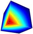
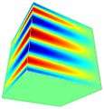
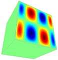
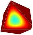
The Fichera problem (also called the Fichera corner problem) is a standard benchmark problem for adaptive FEM codes. One can use it to show the dramatic difference in the performance of standard FEM and the hp-FEM. The problem geometry is a cube with missing corner. The exact solution has a singular gradient (an analogy of infinite stress) at the center. The knowledge of the exact solution makes it possible to calculate the approximation error exactly and thus compare various numerical methods. For illustration, the problem was solved using three different versions of adaptive FEM: with linear elements, quadratic elements, and the hp-FEM.
-

Fichera problem: singular gradient.
-
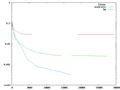
Fichera problem: convergence comparison.
The convergence graphs show the approximation error as a function of the number of degrees of freedom (DOF). By DOF we mean (unknown) parameters that are needed to define the approximation. The number of DOF equals the size of the stiffness matrix. The reader can see in the graphs that the convergence of the hp-FEM is much faster than the convergence of both other methods. Actually, the performance gap is so huge that the linear FEM might not converge at all in reasonable time and the quadratic FEM would need hundreds of thousands or perhaps millions of DOF to reach the accuracy that the hp-FEM attained with approximately 17,000 DOF. Obtaining very accurate results using relatively few DOF is the main strength of the hp-FEM.
Why is hp-FEM so efficient?
Smooth functions can be approximated much more efficiently using large high-order elements than small piecewise-linear ones. This is illustrated in the figure below, where a 1D Poisson equation with zero Dirichlet boundary conditions is solved on two different meshes. The exact solution is the sin function.
- Left: mesh consisting of two linear elements.
- Right: mesh consisting of one quadratic element.

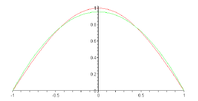
While the number of unknowns is the same in both cases (1 DOF), the errors in the corresponding norm are 0.68 and 0.20, respectively. This means that the quadratic approximation was roughly 3.5-times more efficient than the piecewise-linear one. When we proceed one step further and compare (a) four linear elements to (b) one quartic element (p=4), then both discrete problems will have three DOF but the quartic approximation will be approximately 40-times more efficient. When performing few more steps like this, the reader will see that the efficiency gap opens extremely fast.
On the contrary, small low-order elements can capture small-scale features such as singularities much better than large high-order ones. The hp-FEM is based on an optimal combination of these two approaches which leads to exponential convergence.
What is hp-adaptivity?
Some FEM sites describe hp-adaptivity as a combination of h-adaptivity (splitting elements in space while keeping their polynomial degree fixed) and p-adaptivity (only increasing their polynomial degree). This is not entirely accurate. The hp-adaptivity is significantly different from both h- and p-adaptivity since the hp-refinement of an element can be done in many different ways. Besides a p-refinement, the element can be subdivided in space (as in h-adaptivity), but there are many combinations for the polynomial degrees on the subelements. This is illustrated in the figure on the right. For example, if a triangular or quadrilateral element is subdivided into four subelements where the polynomial degrees are allowed to vary by at most two, then this yields 3^4 = 81 refinement candidates (not considering polynomially anisotropic candidates). Analogously, splitting a hexahedron into eight subelements and varying their polynomial degrees by at most two yields 3^8 = 6,561 refinement candidates. Clearly, standard FEM error estimates providing one constant number per element are not enough to guide automatic hp-adaptivity.
Higher-order shape functions
In standard FEM one only works with shape functions associated with grid vertices (the so-called vertex functions). In contrast to that, in the hp-FEM one moreover regards edge functions (associated with element edges), face functions (corresponding to element faces - 3D only), and bubble functions (higher-order polynomials which vanish on element boundaries). The following images show these functions (restricted to a single element):
-
Vertex function.
-
Edge function.
-
Face function.
-
Bubble function.
Note: all these functions are defined in the entire element interior!
Open source hp-FEM codes
- Concepts: C/C++ hp-FEM/DGFEM/BEM library for elliptic equations developed at SAM, ETH Zurich (Switzerland) and in the group of K. Schmidt at TU Berlin (Germany).
- 2dhp90, 3dhp90: Fortran codes for elliptic problems and Maxwell's equations developed by L. Demkowicz at ICES, UT Austin.
- PHAML: The Parallel Hierarchical Adaptive MultiLevel Project. Finite element software developed at the National Institute for Standards and Technology, USA, for numerical solution of 2D elliptic partial differential equations on distributed memory parallel computers and multicore computers using adaptive mesh refinement and multigrid solution techniques.
- Hermes Project: C/C++/Python library for rapid prototyping of space- and space-time adaptive hp-FEM solvers for a large variety of PDEs and multiphysics PDE systems, developed by the hp-FEM group at the University of Nevada, Reno (USA), Institute of Thermomechanics, Prague (Czech Republic), and the University of West Bohemia in Pilsen (Czech Republic) - with the Agros2D engineering software built on top of the Hermes library.
- PHG: PHG is a toolbox for developing parallel adaptive finite element programs. It's suitable for h-, p- and hp-fem. PHG is currently under active development at State Key Laboratory of Scientific and Engineering Computing, Institute of Computational Mathematics and Scientific/Engineering Computing of Chinese Academy of Sciences(LSEC, CAS, China).PHG deals with conforming tetrahedral meshes and uses bisection for adaptive local mesh refinement and MPI for message passing. PHG has an object oriented design which hides parallelization details and provides common operations on meshes and finite element functions in an abstract way, allowing the users to concentrate on their numerical algorithms.
- Deal.II: deal.II is a free, open source library to solve partial differential equations using the finite element method.
References
- ↑ I. Babuska, B.Q. Guo: The h, p and h-p version of the finite element method: basis theory and applications, Advances in Engineering Software, Volume 15, Issue 3-4, 1992.
- ↑ J.M. Melenk: hp-Finite Element Methods for Singular Perturbations, Springer, 2002
- ↑ C. Schwab: p- and hp- Finite Element Methods: Theory and Applications in Solid and Fluid Mechanics, Oxford University Press, 1998
- ↑ P. Solin: Partial Differential Equations and the Finite Element Method, J. Wiley & Sons, 2005
- ↑ P. Solin, K. Segeth, I. Dolezel: Higher-Order Finite Element Methods, Chapman & Hall/CRC Press, 2003
- ↑ I. Babuska, M. Griebel and J. Pitkaranta, The problem of selecting the shape functions for a p-type finite element, Internat. J. Numer. Methods Engrg. (1989), pp. 1891-1908
- ↑ L. Demkowicz, W. Rachowicz, and Ph. Devloo: A Fully Automatic hp-Adaptivity, Journal of Scientific Computing, 17, Nos 1-3 (2002), 127-155
- ↑ P. Solin, T. Vejchodsky: A Weak Discrete Maximum Principle for hp-FEM, J. Comput. Appl. Math. 209 (2007) 54-65
- ↑ T. Vejchodsky, P. Solin: Discrete Maximum Principle for Higher-Order Finite Elements in 1D, Math. Comput. 76 (2007), 1833 - 1846
- ↑ L. Demkowicz, J. Kurtz, D. Pardo, W. Rachowicz, M. Paszynski, A. Zdunek: Computing with hp-Adaptive Finite Elements, Chapman & Hall/CRC Press, 2007