Fractional Brownian motion
In probability theory, fractional Brownian motion (fBm), also called a fractal Brownian motion, is a generalization of Brownian motion. Unlike classical Brownian motion, the increments of fBm need not be independent. fBm is a continuous-time Gaussian process BH(t) on [0, T], which starts at zero, has expectation zero for all t in [0, T], and has the following covariance function:
![E[B_H(t) B_H (s)]=\tfrac{1}{2} (|t|^{2H}+|s|^{2H}-|t-s|^{2H}),](../I/m/914fd4046e7a501aba142e475493c40be2888036.svg)
where H is a real number in (0, 1), called the Hurst index or Hurst parameter associated with the fractional Brownian motion. The Hurst exponent describes the raggedness of the resultant motion, with a higher value leading to a smoother motion. It was introduced by Mandelbrot & van Ness (1968).
The value of H determines what kind of process the fBm is:
- if H = 1/2 then the process is in fact a Brownian motion or Wiener process;
- if H > 1/2 then the increments of the process are positively correlated;
- if H < 1/2 then the increments of the process are negatively correlated.
The increment process, X(t) = BH(t+1) − BH(t), is known as fractional Gaussian noise.
There is also a generalization of fractional Brownian motion: n-th order fractional Brownian motion, abbreviated as n-fBm.[1] n-fBm is a Gaussian, self-similar, non-stationary process whose increments of order n are stationary. For n = 1, n-fBm is classical fBm.
Like the Brownian motion that it generalizes, fractional Brownian motion is named after 19th century biologist Robert Brown; fractional Gaussian noise is named after mathematician Carl Friedrich Gauss.
Background and definition
Prior to the introduction of the fractional Brownian motion, Lévy (1953) used the Riemann–Liouville fractional integral to define the process

where integration is with respect to the white noise measure dB(s). This integral turns out to be ill-suited to applications of fractional Brownian motion because of its over-emphasis of the origin (Mandelbrot & van Ness 1968, p. 424).
The idea instead is to use a different fractional integral of white noise to define the process: the Weyl integral
![B_H (t) = B_H (0) + \frac{1}{\Gamma(H+1/2)}\left\{\int_{-\infty}^0\left[(t-s)^{H-1/2}-(-s)^{H-1/2}\right]\,dB(s) + \int_0^t (t-s)^{H-1/2}\,dB(s)\right\}](../I/m/443ff3deb2f7ca24cbc0067dba9f05d2d7dcb40d.svg)
for t > 0 (and similarly for t < 0).
The main difference between fractional Brownian motion and regular Brownian motion is that while the increments in Brownian Motion are independent, the opposite is true for fractional Brownian motion. This dependence means that if there is an increasing pattern in the previous steps, then it is likely that the current step will be increasing as well. (If H > 1/2.)
Properties
Self-similarity
The process is self-similar, since in terms of probability distributions:

This property is due to the fact that the covariance function is homogeneous of order 2H and can be considered as a fractal property. Fractional Brownian motion is the only self-similar Gaussian process.
Stationary increments
It has stationary increments:

Long-range dependence
For H > ½ the process exhibits long-range dependence,
![\sum_{n=1}^\infty E[B_H (1)(B_H (n+1)-B_H (n))] = \infty.](../I/m/2c86d29dfcec88c3e0de082abd375a6f914a97c2.svg)
Regularity
Sample-paths are almost nowhere differentiable. However, almost-all trajectories are Hölder continuous of any order strictly less than H: for each such trajectory, for every T > 0 and for every ε > 0 there exists a constant c such that

for 0 < s,t < T.
Dimension
With probability 1, the graph of BH(t) has both Hausdorff dimension and box dimension of 2−H.
Integration
As for regular Brownian motion, one can define stochastic integrals with respect to fractional Brownian motion, usually called "fractional stochastic integrals". In general though, unlike integrals with respect to regular Brownian motion, fractional stochastic integrals are not semimartingales.
Sample paths
Practical computer realisations of an fBm can be generated,[2] although they are only a finite approximation. The sample paths chosen can be thought of as showing discrete sampled points on an fBm process. Three realisations are shown below, each with 1000 points of an fBm with Hurst parameter 0.75.
 "H" = 0.75 realisation 1 |
 "H" = 0.75 realisation 2 |
 "H" = 0.75 realisation 3 |
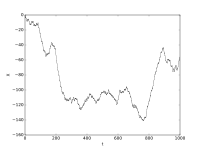
Two realisations are shown below, each showing 1000 points of an fBm, the first with Hurst parameter 0.15, the second with Hurst parameter 0.55, and the third with Hurst parameter 0.95. The higher Hurst parameter is, the more smooth the curve will be.
 "H" = 0.15 |
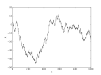 "H" = 0.55 |
 "H" = 0.95 |
Method 1 of simulation
One can simulate sample-paths of an fBm using methods for generating stationary Gaussian processes with known covariance function. The simplest method relies on the Cholesky decomposition method of the covariance matrix (explained below), which on a grid of size has complexity of order . A more complex, but computationally faster method is the circulant embedding method of Dietrich & Newsam (1997).


Suppose we want to simulate the values of the fBM at times using the Cholesky decomposition method.

- Form the matrix where .
- Compute the square root matrix of , i.e. . Loosely speaking, is the "standard deviation" matrix associated to the variance-covariance matrix .
- Construct a vector of n numbers drawn according to a standard Gaussian distribution,
- If we define then yields a sample path of an fBm.


In order to compute , we can use for instance the Cholesky decomposition method. An alternative method uses the eigenvalues of :
- Since is symmetric, positive-definite matrix, it follows that all eigenvalues of satisfy , ().
- Let be the diagonal matrix of the eigenvalues, i.e. where is the Kronecker delta. We define as the diagonal matrix with entries , i.e. .


Note that the result is real-valued because .

- Let an eigenvector associated to the eigenvalue . Define as the matrix whose -th column is the eigenvector .


Note that since the eigenvectors are linearly independent, the matrix is inversible.
- It follows then that because .


Method 2 of simulation
It is also known that [3]

where B is a standard Brownian motion and

Where is the Euler hypergeometric integral.

Say we want simulate an fBm at points .

- Construct a vector of n numbers drawn according to a standard Gaussian distribution.
- Multiply it component-wise by √(T/n) to obtain the increments of a Brownian motion on [0, T]. Denote this vector by .
- For each , compute


The integral may be efficiently computed by Gaussian quadrature. Hypergeometric functions are part of the GNU scientific library.
See also
- Brownian surface
- Autoregressive fractionally integrated moving average
- Multifractal: The generalized framework of fractional Brownian motions.
- Pink noise
- Tweedie distributions
Notes
- ↑ Perrin et al., 2001.
- ↑ Kroese, D.P.; Botev, Z.I. (2014). "Spatial Process Generation". Lectures on Stochastic Geometry, Spatial Statistics and Random Fields, Volume II: Analysis, Modeling and Simulation of Complex Structures, Springer-Verlag, Berlin. arXiv:1308.0399
 .
. - ↑ Stochastic Analysis of the Fractional Brownian Motion,
References
- Beran, J. (1994), Statistics for Long-Memory Processes, Chapman & Hall, ISBN 0-412-04901-5.
- Craigmile P.F. (2003), "Simulating a class of stationary Gaussian processes using the Davies–Harte Algorithm, with application to long memory processes", Journal of Times Series Analysis, 24: 505–511.
- Dieker, T. (2004). Simulation of fractional Brownian motion (PDF) (M.Sc. thesis). Retrieved 29 December 2012.
- Dietrich, C. R.; Newsam, G. N. (1997), "Fast and exact simulation of stationary Gaussian processes through circulant embedding of the covariance matrix.", SIAM Journal on Scientific Computing, 18 (4): 1088–1107, doi:10.1137/s1064827592240555.
- Lévy, P. (1953), Random functions: General theory with special references to Laplacian random functions, University of California Publications in Statistics, 1, pp. 331–390.
- Mandelbrot, B.; van Ness, J.W. (1968), "Fractional Brownian motions, fractional noises and applications", SIAM Review, 10 (4): 422–437, doi:10.1137/1010093, JSTOR 2027184.
- Perrin E. et al. (2001), "nth-order fractional Brownian motion and fractional Gaussian noises", IEEE Transactions on Signal Processing, 49: 1049-1059. doi:10.1109/78.917808
- Samorodnitsky G., Taqqu M.S. (1994), Stable Non-Gaussian Random Processes, Chapter 7: "Self-similar processes" (Chapman & Hall).
Further reading
- Sainty, P. (1992), "Construction of a complex‐valued fractional Brownian motion of order N", Journal of Mathematical Physics, 33: 3128, doi:10.1063/1.529976.