Gaussian quadrature


In numerical analysis, a quadrature rule is an approximation of the definite integral of a function, usually stated as a weighted sum of function values at specified points within the domain of integration. (See numerical integration for more on quadrature rules.) An n-point Gaussian quadrature rule, named after Carl Friedrich Gauss, is a quadrature rule constructed to yield an exact result for polynomials of degree 2n − 1 or less by a suitable choice of the points xi and weights wi for i = 1, ..., n. The domain of integration for such a rule is conventionally taken as [−1, 1], so the rule is stated as

Gaussian quadrature as above will only produce good results if the function f(x) is well approximated by a polynomial function within the range [−1, 1]. The method is not, for example, suitable for functions with singularities. However, if the integrated function can be written as , where g(x) is approximately polynomial and ω(x) is known, then alternative weights and points that depend on the weighting function ω(x) may give better results, where


Common weighting functions include (Chebyshev–Gauss) and (Gauss–Hermite).


It can be shown (see Press, et al., or Stoer and Bulirsch) that the evaluation points xi are just the roots of a polynomial belonging to a class of orthogonal polynomials.
Gauss–Legendre quadrature
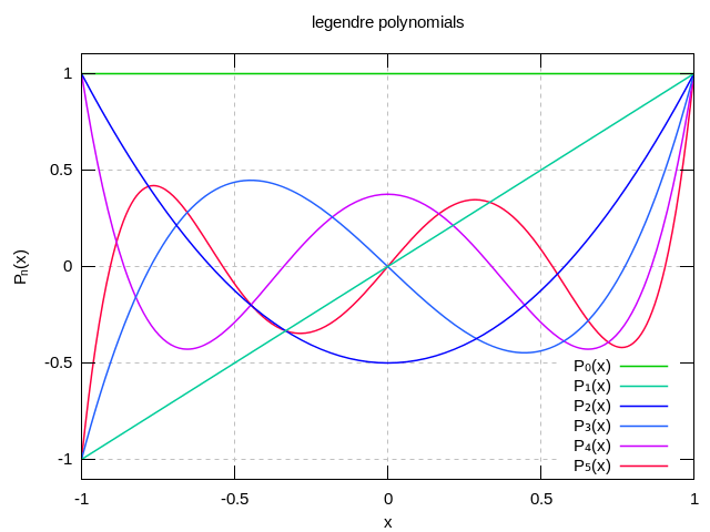
For the simplest integration problem stated above, i.e. with , the associated polynomials are Legendre polynomials, Pn(x), and the method is usually known as Gauss–Legendre quadrature. With the n-th polynomial normalized to give Pn(1) = 1, the i-th Gauss node, xi, is the i-th root of Pn; its weight is given by (Abramowitz & Stegun 1972, p. 887)

![w_{i}={\frac {2}{\left(1-x_{i}^{2}\right)[P'_{n}(x_{i})]^{2}}}.](../I/m/ced974d823852285fd484f2fb39ae82744f0637f.svg)
Some low-order rules for solving the integration problem are listed below (over interval [−1, 1], see the section below for other intervals).
| Number of points, n | Points, xi | Weights, wi |
|---|---|---|
| 1 | 0 | 2 |
| 2 | 1 | |
| 3 | 0 | |
| 4 | ||
| 5 | 0 | |


Change of interval
An integral over [a, b] must be changed into an integral over [−1, 1] before applying the Gaussian quadrature rule. This change of interval can be done in the following way:

Applying the Gaussian quadrature rule then results in the following approximation:

Other forms
The integration problem can be expressed in a slightly more general way by introducing a positive weight function ω into the integrand, and allowing an interval other than [−1, 1]. That is, the problem is to calculate

for some choices of a, b, and ω. For a = −1, b = 1, and ω(x) = 1, the problem is the same as that considered above. Other choices lead to other integration rules. Some of these are tabulated below. Equation numbers are given for Abramowitz and Stegun (A & S).
| Interval | ω(x) | Orthogonal polynomials | A & S | For more information, see ... |
|---|---|---|---|---|
| [−1, 1] | 1 | Legendre polynomials | 25.4.29 | See Gauss–Legendre quadrature above |
| (−1, 1) | Jacobi polynomials | 25.4.33 (β = 0) | Gauss–Jacobi quadrature | |
| (−1, 1) | Chebyshev polynomials (first kind) | 25.4.38 | Chebyshev–Gauss quadrature | |
| [−1, 1] | Chebyshev polynomials (second kind) | 25.4.40 | Chebyshev–Gauss quadrature | |
| [0, ∞) | Laguerre polynomials | 25.4.45 | Gauss–Laguerre quadrature | |
| [0, ∞) | Generalized Laguerre polynomials | Gauss–Laguerre quadrature | ||
| (−∞, ∞) | Hermite polynomials | 25.4.46 | Gauss–Hermite quadrature |


Fundamental theorem
Let pn be a nontrivial polynomial of degree n such that

If we pick the n nodes xi to be the zeros of pn, then there exist n weights wi which make the Gauss-quadrature computed integral exact for all polynomials h(x) of degree 2n − 1 or less. Furthermore, all these nodes xi will lie in the open interval (a, b) (Stoer & Bulirsch 2002, pp. 172–175).
The polynomial pn is said to be an orthogonal polynomial of degree n associated to the weight function ω(x). It is unique up to a constant normalization factor. The idea underlying the proof is that, because of its sufficiently low degree, h(x) can be divided by to produce a quotient q(x) of degree strictly lower than n, and a remainder r(x) of still lower degree, so that both will be orthogonal to , by the defining property of . Thus


Because of the choice of nodes xi, the corresponding relation

holds also. The exactness of the computed integral for then follows from corresponding exactness for polynomials of degree only n or less (as is ).


General formula for the weights
The weights can be expressed as
- (1)

where is the coefficient of in . To prove this, note that using Lagrange interpolation one can express r(x) in terms of as


because r(x) has degree less than n and is thus fixed by the values it attains at n different points. Multiplying both sides by ω(x) and integrating from a to b yields

The weights wi are thus given by

This integral expression for can be expressed in terms of the orthogonal polynomials and as follows.


We can write

where is the coefficient of in . Taking the limit of x to yields using L'Hôpital's rule


We can thus write the integral expression for the weights as
- ---------(2)

In the integrand, writing

yields

provided , because


is a polynomial of degree k-1 which is then orthogonal to . So, if q(x) is a polynomial of at most nth degree we have

We can evaluate the integral on the right hand side for as follows. Because is a polynomial of degree n-1, we have


where s(x) is a polynomial of degree . Since s(x) is orthogonal to we have


We can then write

The term in the brackets is a polynomial of degree , which is therefore orthogonal to . The integral can thus be written as

According to Eq. (2), the weights are obtained by dividing this by and that yields the expression in Eq. (1).

can also be expressed in terms of the orthogonal polynomials and now . In the 3-term recurrence relation the term with vanishes, so in Eq. (1) can be replaced by .


Proof that the weights are positive
Consider the following polynomial of degree 2n-2

where as above the xj are the roots of the polynomial . Since the degree of f(x) is less than 2n-1, the Gaussian quadrature formula involving the weights and nodes obtained from applies. Since for j not equal to i, we have


Since both and f(x) are non-negative functions, it follows that .


Computation of Gaussian quadrature rules
For computing the nodes xi and weights wi of Gaussian quadrature rules, the fundamental tool is the three-term recurrence relation satisfied by the set of orthogonal polynomials associated to the corresponding weight function. For n points, these nodes and weights can be computed in O(n2) operations by an algorithm derived by Gautschi (1968).
Gautschi's theorem
Gautschi's theorem (Gautschi, 1968) states that orthogonal polynomials with for for a scalar product , degree and leading coefficient one (i.e. monic orthogonal polynomials) satisfy the recurrence relation


and scalar product defined

for where n is the maximal degree which can be taken to be infinity, and where . First of all, the polynomials defined by the recurrence relation starting with have leading coefficient one and correct degree. Given the starting point by , the orthogonality of can be shown by induction. For one has


Now if are orthogonal, then also , because in


all scalar products vanish except for the first one and the one where meets the same orthogonal polynomial. Therefore,


However, if the scalar product satisfies (which is the case for Gaussian quadrature), the recurrence relation reduces to a three-term recurrence relation: For is a polynomial of degree less or equal to r − 1. On the other hand, is orthogonal to every polynomial of degree less or equal to r − 1. Therefore, one has and for s < r − 1. The recurrence relation then simplifies to


or

(with the convention ) where


(the last because of , since differs from by a degree less than r).


The Golub-Welsch algorithm
The three-term recurrence relation can be written in the matrix form where , is the th standard basis vector, i.e. , and J is the so-called Jacobi matrix:

![{\tilde {P}}=[p_{0}(x),p_{1}(x),...,p_{n-1}(x)]^{T}](../I/m/74b8c6e90f9adbf403545cad62f5ea7c0d6a59e8.svg)


![\mathbf {e} _{n}=[0,...,0,1]^{T}](../I/m/e7c1f8654f52216e6f6b9470d960d211ed0433b7.svg)

The zeros of the polynomials up to degree n which are used as nodes for the Gaussian quadrature can be found by computing the eigenvalues of this tridiagonal matrix. This procedure is known as Golub–Welsch algorithm.

For computing the weights and nodes, it is preferable to consider the symmetric tridiagonal matrix with elements


J and are similar matrices and therefore have the same eigenvalues (the nodes). The weights can be computed from the corresponding eigenvectors: If is a normalized eigenvector (i.e., an eigenvector with euclidean norm equal to one) associated to the eigenvalue xj, the corresponding weight can be computed from the first component of this eigenvector, namely:


where is the integral of the weight function


See, for instance, (Gil, Segura & Temme 2007) for further details.
Error estimates
The error of a Gaussian quadrature rule can be stated as follows (Stoer & Bulirsch 2002, Thm 3.6.24). For an integrand which has 2n continuous derivatives,

for some ξ in (a, b), where pn is the monic (i.e. the leading coefficient is 1) orthogonal polynomial of degree n and where

In the important special case of ω(x) = 1, we have the error estimate (Kahaner, Moler & Nash 1989, §5.2)
![{\frac {(b-a)^{2n+1}(n!)^{4}}{(2n+1)[(2n)!]^{3}}}f^{(2n)}(\xi ),\qquad a<\xi <b.](../I/m/d6e9f68af83c7073f2b018e03aa2a18ac5295f0d.svg)
Stoer and Bulirsch remark that this error estimate is inconvenient in practice, since it may be difficult to estimate the order 2n derivative, and furthermore the actual error may be much less than a bound established by the derivative. Another approach is to use two Gaussian quadrature rules of different orders, and to estimate the error as the difference between the two results. For this purpose, Gauss–Kronrod quadrature rules can be useful.
Gauss–Kronrod rules
If the interval [a, b] is subdivided, the Gauss evaluation points of the new subintervals never coincide with the previous evaluation points (except at zero for odd numbers), and thus the integrand must be evaluated at every point. Gauss–Kronrod rules are extensions of Gauss quadrature rules generated by adding n + 1 points to an n-point rule in such a way that the resulting rule is of order 2n + 1. This allows for computing higher-order estimates while re-using the function values of a lower-order estimate. The difference between a Gauss quadrature rule and its Kronrod extension are often used as an estimate of the approximation error.
Gauss–Lobatto rules
Also known as Lobatto quadrature (Abramowitz & Stegun 1972, p. 888), named after Dutch mathematician Rehuel Lobatto. It is similar to Gaussian quadrature with the following differences:
- The integration points include the end points of the integration interval.
- It is accurate for polynomials up to degree 2n–3, where n is the number of integration points (Quarteroni, Sacco & Saleri 2000).
Lobatto quadrature of function f(x) on interval [−1, 1]:
![\int _{-1}^{1}{f(x)\,dx}={\frac {2}{n(n-1)}}[f(1)+f(-1)]+\sum _{i=2}^{n-1}{w_{i}f(x_{i})}+R_{n}.](../I/m/debe72ac248f8ae18af6b8814511b7068487ba24.svg)
Abscissas: xi is the st zero of .


Weights:
![w_{i}={\frac {2}{n(n-1)[P_{n-1}(x_{i})]^{2}}},\qquad x_{i}\neq \pm 1.](../I/m/9391d8ca83a478f77c33872c9140942612d57c13.svg)
Remainder:
![R_{n}={\frac {-n(n-1)^{3}2^{2n-1}[(n-2)!]^{4}}{(2n-1)[(2n-2)!]^{3}}}f^{(2n-2)}(\xi ),\qquad -1<\xi <1.](../I/m/791cc0d39c2673b93cb28fbc3e5e49184ef714d9.svg)
Some of the weights are:
| Number of points, n | Points, xi | Weights, wi |
|---|---|---|


See also
References
- Abramowitz, Milton; Stegun, Irene Ann, eds. (1983) [June 1964]. "Chapter 25.4, Integration". Handbook of Mathematical Functions with Formulas, Graphs, and Mathematical Tables. Applied Mathematics Series. 55 (Ninth reprint with additional corrections of tenth original printing with corrections (December 1972); first ed.). Washington D.C., USA; New York, USA: United States Department of Commerce, National Bureau of Standards; Dover Publications. ISBN 0-486-61272-4. LCCN 64-60036. MR 0167642. ISBN 978-0-486-61272-0. LCCN 65-12253.
- Anderson, Donald G. (1965). "Gaussian quadrature formulae for ". Math. Comp. 19 (91): 477–481. doi:10.1090/s0025-5718-1965-0178569-1.
- Golub, Gene H.; Welsch, John H. (1969), "Calculation of Gauss Quadrature Rules", Mathematics of Computation, 23 (106): 221–230, doi:10.1090/S0025-5718-69-99647-1, JSTOR 2004418
- Gautschi, Walter (1968). "Construction of Gauss–Christoffel Quadrature Formulas". Math. Comp. 22 (102). pp. 251–270. doi:10.1090/S0025-5718-1968-0228171-0. MR 0228171.
- Gautschi, Walter (1970). "On the construction of Gaussian quadrature rules from modified moments". Math. Comp. 24. pp. 245–260. doi:10.1090/S0025-5718-1970-0285117-6. MR 0285177.
- Piessens, R. (1971). "Gaussian quadrature formulas for the numerical integration of Bromwich's integral and the inversion of the laplace transform". J. Eng. Math. 5 (1). pp. 1–9. doi:10.1007/BF01535429.
- Danloy, Bernard (1973). "Numerical construction of Gaussian quadrature formulas for and ". Math. Comp. 27 (124). pp. 861–869. doi:10.1090/S0025-5718-1973-0331730-X. MR 0331730.
- Kahaner, David; Moler, Cleve; Nash, Stephen (1989), Numerical Methods and Software, Prentice-Hall, ISBN 978-0-13-627258-8
- Sagar, Robin P. (1991). "A Gaussian quadrature for the calculation of generalized Fermi-Dirac integrals". Comp. Phys. Commun. 66 (2-3): 271–275. Bibcode:1991CoPhC..66..271S. doi:10.1016/0010-4655(91)90076-W.
- Yakimiw, E. (1996). "Accurate computation of weights in classical Gauss-Christoffel quadrature rules". J. Comp. Phys. 129: 406–430. Bibcode:1996JCoPh.129..406Y. doi:10.1006/jcph.1996.0258.
- Laurie, Dirk P. (1999), "Accurate recovery of recursion coefficients from Gaussian quadrature formulas", J. Comp. Appl. Math., 112 (1-2): 165–180, doi:10.1016/S0377-0427(99)00228-9
- Laurie, Dirk P. (2001). "Computation of Gauss-type quadrature formulas". J. Comp. Appl. Math. 127 (1-2): 201–217. Bibcode:2001JCoAM.127..201L. doi:10.1016/S0377-0427(00)00506-9.
- Stoer, Josef; Bulirsch, Roland (2002), Introduction to Numerical Analysis (3rd ed.), Springer, ISBN 978-0-387-95452-3.
- Temme, Nico M. (2010), "§3.5(v): Gauss Quadrature", in Olver, Frank W. J.; Lozier, Daniel M.; Boisvert, Ronald F.; Clark, Charles W., NIST Handbook of Mathematical Functions, Cambridge University Press, ISBN 978-0521192255, MR 2723248
- Press, WH; Teukolsky, SA; Vetterling, WT; Flannery, BP (2007), "Section 4.6. Gaussian Quadratures and Orthogonal Polynomials", Numerical Recipes: The Art of Scientific Computing (3rd ed.), New York: Cambridge University Press, ISBN 978-0-521-88068-8
- Gil, Amparo; Segura, Javier; Temme, Nico M. (2007), "§5.3: Gauss quadrature", Numerical Methods for Special Functions, SIAM, ISBN 978-0-89871-634-4
- Quarteroni, Alfio; Sacco, Riccardo; Saleri, Fausto (2000). Numerical Mathematics. New York: Springer-Verlag. pp. 422, 425. ISBN 0-387-98959-5.


External links
- Hazewinkel, Michiel, ed. (2001), "Gauss quadrature formula", Encyclopedia of Mathematics, Springer, ISBN 978-1-55608-010-4
- ALGLIB contains a collection of algorithms for numerical integration (in C# / C++ / Delphi / Visual Basic / etc.)
- GNU Scientific Library — includes C version of QUADPACK algorithms (see also GNU Scientific Library)
- From Lobatto Quadrature to the Euler constant e
- Gaussian Quadrature Rule of Integration – Notes, PPT, Matlab, Mathematica, Maple, Mathcad at Holistic Numerical Methods Institute
- Weisstein, Eric W. "Legendre-Gauss Quadrature". MathWorld.
- Gaussian Quadrature by Chris Maes and Anton Antonov, Wolfram Demonstrations Project.
- Tabulated weights and abscissae with Mathematica source code, high precision (16 and 256 decimal places) Legendre-Gaussian quadrature weights and abscissas, for n=2 through n=64, with Mathematica source code.
- Mathematica source code distributed under the GNU LGPL for abscissas and weights generation for arbitrary weighting functions W(x), integration domains and precisions.