Zipf's law

Zipf's law
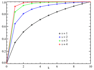
Probability mass function Zipf PMF for N = 10 on a log–log scale. The horizontal axis is the index k . (Note that the function is only defined at integer values of k. The connecting lines do not indicate continuity.)
Cumulative distribution function Zipf CDF for N = 10. The horizontal axis is the index k . (Note that the function is only defined at integer values of k. The connecting lines do not indicate continuity.)
Parameters	$s>1\,$ (real) $N\in \{1,2,3\ldots \}$ (integer)
Support	$k\in \{1,2,\ldots ,N\}$
pmf	${\frac {1/k^{s}}{H_{N,s}}}$ where H_N,s is the Nth generalized harmonic number
CDF	${\frac {H_{k,s}}{H_{N,s}}}$
Mean	${\frac {H_{N,s-1}}{H_{N,s}}}$
Mode	$1\,$
Entropy	${\frac {s}{H_{N,s}}}\sum _{k=1}^{N}{\frac {\ln(k)}{k^{s}}}+\ln(H_{N,s})$
MGF	${\frac {1}{H_{N,s}}}\sum _{n=1}^{N}{\frac {e^{nt}}{n^{s}}}$
CF	${\frac {1}{H_{N,s}}}\sum _{n=1}^{N}{\frac {e^{int}}{n^{s}}}$

Zipf's law /ˈzɪf/ is an empirical law formulated using mathematical statistics that refers to the fact that many types of data studied in the physical and social sciences can be approximated with a Zipfian distribution, one of a family of related discrete power law probability distributions. The law is named after the American linguist George Kingsley Zipf (1902–1950), who popularized it and sought to explain it (Zipf 1935, 1949), though he did not claim to have originated it.^[1] The French stenographer Jean-Baptiste Estoup (1868–1950) appears to have noticed the regularity before Zipf.^[2] It was also noted in 1913 by German physicist Felix Auerbach^[3] (1856–1933).

Motivation

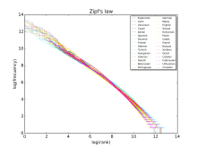
Zipf's law states that given some corpus of natural language utterances, the frequency of any word is inversely proportional to its rank in the frequency table. Thus the most frequent word will occur approximately twice as often as the second most frequent word, three times as often as the third most frequent word, etc.: the rank-frequency distribution is an inverse relation. For example, in the Brown Corpus of American English text, the word "the" is the most frequently occurring word, and by itself accounts for nearly 7% of all word occurrences (69,971 out of slightly over 1 million). True to Zipf's Law, the second-place word "of" accounts for slightly over 3.5% of words (36,411 occurrences), followed by "and" (28,852). Only 135 vocabulary items are needed to account for half the Brown Corpus.^[4]

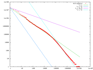
The same relationship occurs in many other rankings unrelated to language, such as the population ranks of cities in various countries, corporation sizes, income rankings, ranks of number of people watching the same TV channel,^[5] and so on. The appearance of the distribution in rankings of cities by population was first noticed by Felix Auerbach in 1913.^[3] Empirically, a data set can be tested to see whether Zipf's law applies by checking the goodness of fit of an empirical distribution to the hypothesized power law distribution with a Kolmogorov-Smirnov test, and then comparing the (log) likelihood ratio of the power law distribution to alternative distributions like an exponential distribution or lognormal distribution.^[6] When Zipf's law is checked for cities, a better fit has been found with exponent s = 1.07; i.e. the $n^{th}$ largest settlement is ${\frac {1}{n^{1.07}}}$ the size of the largest settlement. While Zipf's law holds for the upper tail of the distribution, the entire distribution of cities is log-normal and follows Gibrat's law.^[7] Both laws are consistent because a log-normal tail can typically not be distinguished from a Pareto (Zipf) tail.

Theoretical review

Zipf's law is most easily observed by plotting the data on a log-log graph, with the axes being log (rank order) and log (frequency). For example, the word "the" (as described above) would appear at x = log(1), y = log(69971). It is also possible to plot reciprocal rank against frequency or reciprocal frequency or interword interval against rank.^[1] The data conform to Zipf's law to the extent that the plot is linear.

Formally, let:

N be the number of elements;
k be their rank;
s be the value of the exponent characterizing the distribution.

Zipf's law then predicts that out of a population of N elements, the frequency of elements of rank k, f(k;s,N), is:

f(k;s,N)={\frac {1/k^{s}}{\sum _{n=1}^{N}(1/n^{s})}}

Zipf's law holds if the number of elements with a given frequency is a random variable with power law distribution $p(f)=\alpha f^{-1-1/s}.$ ^[8]

It has been claimed that this representation of Zipf's law is more suitable for statistical testing, and in this way it has been analyzed in more than 30,000 English texts. The goodness-of-fit tests yield that only about 15% of the texts are statistically compatible with this form of Zipf's law. Slight variations in the definition of Zipf's law can increase this percentage up to close to 50%.^[9]

In the example of the frequency of words in the English language, N is the number of words in the English language and, if we use the classic version of Zipf's law, the exponent s is 1. f(k; s,N) will then be the fraction of the time the kth most common word occurs.

The law may also be written:

f(k;s,N)={\frac {1}{k^{s}H_{N,s}}}

where H_N,s is the Nth generalized harmonic number.

The simplest case of Zipf's law is a "¹⁄_f function". Given a set of Zipfian distributed frequencies, sorted from most common to least common, the second most common frequency will occur ½ as often as the first. The third most common frequency will occur ⅓ as often as the first. The n^th most common frequency will occur ¹⁄_n as often as the first. However, this cannot hold exactly, because items must occur an integer number of times; there cannot be 2.5 occurrences of a word. Nevertheless, over fairly wide ranges, and to a fairly good approximation, many natural phenomena obey Zipf's law.

Mathematically, the sum of all relative frequencies in a Zipf distribution is equal to the harmonic series, and

\sum _{n=1}^{\infty }{\frac {1}{n}}=\infty .\!

In human languages, word frequencies have a very heavy-tailed distribution, and can therefore be modeled reasonably well by a Zipf distribution with an s close to 1.

As long as the exponent s exceeds 1, it is possible for such a law to hold with infinitely many words, since if s > 1 then

\zeta (s)=\sum _{n=1}^{\infty }{\frac {1}{n^{s}}}<\infty .\!

where ζ is Riemann's zeta function.

Statistical explanation

A plot of the rank versus frequency for the first 10 million words in 30 Wikipedias (dumps from October 2015) in a log-log scale.

Although Zipf’s Law holds for most languages, even for non-natural languages like Esperanto,^[10] the reason is still not well understood.^[11] However, it may be partially explained by the statistical analysis of randomly generated texts. Wentian Li has shown that in a document in which each character has been chosen randomly from a uniform distribution of all letters (plus a space character), the "words" follow the general trend of Zipf's law (appearing approximately linear on log-log plot).^[12] Vitold Belevitch in a paper, On the Statistical Laws of Linguistic Distribution offered a mathematical derivation. He took a large class of well-behaved statistical distributions (not only the normal distribution) and expressed them in terms of rank. He then expanded each expression into a Taylor series. In every case Belevitch obtained the remarkable result that a first-order truncation of the series resulted in Zipf's law. Further, a second-order truncation of the Taylor series resulted in Mandelbrot's law.^[13]^[14]

The principle of least effort is another possible explanation: Zipf himself proposed that neither speakers nor hearers using a given language want to work any harder than necessary to reach understanding, and the process that results in approximately equal distribution of effort leads to the observed Zipf distribution.^[15]^[16]

Similarly, preferential attachment (intuitively, "the rich get richer" or "success breeds success") that results in the Yule-Simon distribution has been shown to fit word frequency versus rank in language^[17] and population versus city rank^[18] better than Zipf's law. It was originally derived to explain population versus rank in species by Yule, and applied to cities by Simon.

Related laws

A plot of word frequency in Wikipedia (November 27, 2006). The plot is in log-log coordinates. x is rank of a word in the frequency table; y is the total number of the word’s occurrences. Most popular words are "the", "of" and "and", as expected. Zipf's law corresponds to the middle linear portion of the curve, roughly following the green (1/x) line, while the early part is closer to the magenta (1/"x^0.5") line while the later part is closer to the cyan (1/"(k+x)^2.0") line. These lines correspond to three distinct parameterizations of the Zipf-Mandelbrot distribution, overall a broken power law with three segments: a head, middle, and tail.

Zipf's law in fact refers more generally to frequency distributions of "rank data," in which the relative frequency of the nth-ranked item is given by the Zeta distribution, 1/(n^sζ(s)), where the parameter s > 1 indexes the members of this family of probability distributions. Indeed, Zipf's law is sometimes synonymous with "zeta distribution," since probability distributions are sometimes called "laws". This distribution is sometimes called the Zipfian distribution.

A generalization of Zipf's law is the Zipf–Mandelbrot law, proposed by Benoît Mandelbrot, whose frequencies are:

f(k;N,q,s)={\frac {[{\mbox{constant}}]}{(k+q)^{s}}}.\,

The "constant" is the reciprocal of the Hurwitz zeta function evaluated at s. In practice, as easily observable in distribution plots for large corpora, the observed distribution can better be modelled as a sum of separate distributions for different subsets or subtypes of words that follow different parameterizations of the Zipf-Mandelbrot distribution, in particular the closed class of functional words exhibit "s" lower than 1, while open-ended vocabulary growth with document size and corpus size require "s" greater than 1 for convergence of the Generalized Harmonic Series.^[1]

Zipfian distributions can be obtained from Pareto distributions by an exchange of variables.^[8]

The Zipf distribution is sometimes called the discrete Pareto distribution^[19] because it is analogous to the continuous Pareto distribution in the same way that the discrete uniform distribution is analogous to the continuous uniform distribution.

The tail frequencies of the Yule–Simon distribution are approximately

f(k;\rho )\approx {\frac {[{\mbox{constant}}]}{k^{\rho +1}}}

for any choice of ρ > 0.

In the parabolic fractal distribution, the logarithm of the frequency is a quadratic polynomial of the logarithm of the rank. This can markedly improve the fit over a simple power-law relationship.^[20] Like fractal dimension, it is possible to calculate Zipf dimension, which is a useful parameter in the analysis of texts.^[21]

It has been argued that Benford's law is a special bounded case of Zipf's law,^[20] with the connection between these two laws being explained by their both originating from scale invariant functional relations from statistical physics and critical phenomena.^[22] The ratios of probabilities in Benford's law are not constant. The leading digits of data satisfying Zipf's law with s = 1 satisfy Benford's law.

$n$	Benford's law: $P(n)=$ $\log _{10}(n+1)-\log _{10}(n)$	${\tfrac {\log(P(n)/P(n-1))}{\log(n/(n-1))}}$
1	0.30103000
2	0.17609126	-0.7735840
3	0.12493874	-0.8463832
4	0.09691001	-0.8830605
5	0.07918125	-0.9054412
6	0.06694679	-0.9205788
7	0.05799195	-0.9315169
8	0.05115252	-0.9397966
9	0.04575749	-0.9462848

References

1 2 3 Powers, David M W (1998). "Applications and explanations of Zipf's law". Association for Computational Linguistics: 151–160. External link in |title= (help)
↑ Christopher D. Manning, Hinrich Schütze Foundations of Statistical Natural Language Processing, MIT Press (1999), ISBN 978-0-262-13360-9, p. 24
1 2 Auerbach F. (1913) Das Gesetz der Bevölkerungskonzentration. Petermann’s Geographische Mitteilungen 59, 74–76
↑ Fagan, Stephen; Gençay, Ramazan (2010), "An introduction to textual econometrics", in Ullah, Aman; Giles, David E. A., Handbook of Empirical Economics and Finance, CRC Press, pp. 133–153, ISBN 9781420070361 . P. 139: "For example, in the Brown Corpus, consisting of over one million words, half of the word volume consists of repeated uses of only 135 words."
↑ M. Eriksson, S.M. Hasibur Rahman, F. Fraille, M. Sjöström, ”Efficient Interactive Multicast over DVB-T2 - Utilizing Dynamic SFNs and PARPS”, 2013 IEEE International Conference on Computer and Information Technology (BMSB’13), London, UK, June 2013. Suggests a heterogeneous Zipf-law TV channel-selection model
↑ Clauset, A., Shalizi, C. R., & Newman, M. E. J. (2009). Power-Law Distributions in Empirical Data. SIAM Review, 51(4), 661–703. doi:10.1137/070710111
↑ Eeckhout J. (2004), Gibrat's law for (All) Cities. American Economic Review 94(5), 1429-1451.
1 2 Adamic, Lada A. (2000) "Zipf, Power-laws, and Pareto - a ranking tutorial", originally published at http://www.parc.xerox.com/istl/groups/iea/papers/ranking/ranking.html
↑ Moreno-Sánchez, I; Font-Clos, F; Corral, A (2016). "Large-Scale Analysis of Zipf's Law in English Texts". PLoS ONE. doi:10.1371/journal.pone.0147073.
↑ Bill Manaris; Luca Pellicoro; George Pothering; Harland Hodges (13 February 2006). INVESTIGATING ESPERANTO’S STATISTICAL PROPORTIONS RELATIVE TO OTHER LANGUAGES USING NEURAL NETWORKS AND ZIPF’S LAW (PDF). Artificial Intelligence and Applications. Innsbruck, Austria. pp. 102–108.
↑ Léon Brillouin, La science et la théorie de l'information, 1959, réédité en 1988, traduction anglaise rééditée en 2004
↑ Wentian Li (1992). "Random Texts Exhibit Zipf's-Law-Like Word Frequency Distribution". IEEE Transactions on Information Theory. 38 (6): 1842–1845. doi:10.1109/18.165464.
↑ Neumann, Peter G. "Statistical metalinguistics and Zipf/Pareto/Mandelbrot", SRI International Computer Science Laboratory, accessed and archived 29 May 2011.
↑ Belevitch V (18 December 1959). "On the statistical laws of linguistic distributions". Annales de la Société Scientifique de Bruxelles. I. 73: 310–326.
↑ Zipf GK (1949). Human Behavior and the Principle of Least Effort. Cambridge, Massachusetts: Addison-Wesley. p. 1.
↑ Ramon Ferrer i Cancho & Ricard V. Sole (2003). "Least effort and the origins of scaling in human language". Proceedings of the National Academy of Sciences of the United States of America. 100 (3): 788–791. doi:10.1073/pnas.0335980100. PMC 298679. PMID 12540826.
↑ http://arxiv.org/pdf/1412.4846.pdf
↑ http://arxiv.org/pdf/1506.08535.pdf
↑ N. L. Johnson; S. Kotz & A. W. Kemp (1992). Univariate Discrete Distributions (second ed.). New York: John Wiley & Sons, Inc. ISBN 0-471-54897-9. , p. 466.
1 2 Johan Gerard van der Galien (2003-11-08). "Factorial randomness: the Laws of Benford and Zipf with respect to the first digit distribution of the factor sequence from the natural numbers". Retrieved 8 July 2016.
↑ Ali Eftekhari (2006) Fractal geometry of texts. Journal of Quantitative Linguistic 13(2-3): 177 – 193.
↑ L. Pietronero, E. Tosatti, V. Tosatti, A. Vespignani (2001) Explaining the uneven distribution of numbers in nature: The laws of Benford and Zipf. Physica A 293: 297 – 304.

External links

Wikimedia Commons has media related to Zipf's law.

Strogatz, Steven (2009-05-29). "Guest Column: Math and the City". The New York Times. Retrieved 2009-05-29. —An article on Zipf's law applied to city populations
Seeing Around Corners (Artificial societies turn up Zipf's law)
PlanetMath article on Zipf's law
Distributions de type "fractal parabolique" dans la Nature (French, with English summary)
An analysis of income distribution
Zipf List of French words
Zipf list for English, French, Spanish, Italian, Swedish, Icelandic, Latin, Portuguese and Finnish from Gutenberg Project and online calculator to rank words in texts
Citations and the Zipf–Mandelbrot's law
Zipf's Law for U.S. Cities by Fiona Maclachlan, Wolfram Demonstrations Project.
Weisstein, Eric W. "Zipf's Law". MathWorld.

Probability distributions

List

Discrete univariate with finite support	Benford Bernoulli beta-binomial binomial categorical hypergeometric Poisson binomial Rademacher discrete uniform Zipf Zipf–Mandelbrot

Discrete univariate with infinite support	beta negative binomial Borel Conway–Maxwell–Poisson discrete phase-type Delaporte extended negative binomial Gauss–Kuzmin geometric logarithmic negative binomial parabolic fractal Poisson Skellam Yule–Simon zeta

Continuous univariate supported on a bounded interval	arcsine ARGUS Balding–Nichols Bates beta beta rectangular Irwin–Hall Kumaraswamy logit-normal noncentral beta raised cosine reciprocal triangular U-quadratic uniform Wigner semicircle

Continuous univariate supported on a semi-infinite interval	Benini Benktander 1st kind Benktander 2nd kind beta prime Burr chi-squared chi Dagum Davis exponential-logarithmic Erlang exponential F folded normal Flory–Schulz Fréchet gamma gamma/Gompertz generalized inverse Gaussian Gompertz half-logistic half-normal Hotelling's T-squared hyper-Erlang hyperexponential hypoexponential inverse chi-squared scaled inverse chi-squared inverse Gaussian inverse gamma Kolmogorov Lévy log-Cauchy log-Laplace log-logistic log-normal Lomax matrix-exponential Maxwell–Boltzmann Maxwell–Jüttner Mittag-Leffler Nakagami noncentral chi-squared Pareto phase-type poly-Weibull Rayleigh relativistic Breit–Wigner Rice shifted Gompertz truncated normal type-2 Gumbel Weibull Discrete Weibull Wilks's lambda

Continuous univariate supported on the whole real line	Cauchy exponential power Fisher's z Gaussian q generalized normal generalized hyperbolic geometric stable Gumbel Holtsmark hyperbolic secant Johnson's S_U Landau Laplace asymmetric Laplace logistic noncentral t normal (Gaussian) normal-inverse Gaussian skew normal slash stable Student's t type-1 Gumbel Tracy–Widom variance-gamma Voigt

Continuous univariate with support whose type varies	generalized extreme value generalized Pareto Tukey lambda q-Gaussian q-exponential q-Weibull shifted log-logistic

Mixed continuous-discrete univariate	rectified Gaussian

Multivariate (joint)	Discrete Ewens multinomial Dirichlet-multinomial negative multinomial Continuous Dirichlet generalized Dirichlet multivariate normal multivariate stable multivariate t normal-inverse-gamma normal-gamma Matrix-valued inverse matrix gamma inverse-Wishart matrix normal matrix t matrix gamma normal-inverse-Wishart normal-Wishart Wishart

Directional	Univariate (circular) directional Circular uniform univariate von Mises wrapped normal wrapped Cauchy wrapped exponential wrapped asymmetric Laplace wrapped Lévy Bivariate (spherical) Kent Bivariate (toroidal) bivariate von Mises Multivariate von Mises–Fisher Bingham

Degenerate and singular	Degenerate Dirac delta function Singular Cantor

Families	Circular compound Poisson elliptical exponential natural exponential location-scale maximum entropy mixture Pearson Tweedie wrapped

Authority control	GND: 4190937-9

This article is issued from Wikipedia - version of the 12/3/2016. The text is available under the Creative Commons Attribution/Share Alike but additional terms may apply for the media files.