Walker circulation
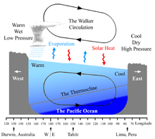
The Walker circulation, also known as the Walker cell, is a conceptual model of the air flow in the tropics in the lower atmosphere (troposphere). According to this model, parcels of air follow a closed circulation in the zonal and vertical directions. This circulation, which is roughly consistent with observations, is caused by differences in heat distribution between ocean and land. It was discovered by Gilbert Walker. In addition to motions in the zonal and vertical direction the tropical atmosphere also has considerable motion in the meridional direction as part of, for example, the Hadley Circulation.
Walker's methodology
Gilbert Walker was an established applied mathematician at the University of Cambridge when he became director-general of observatories in India in 1904.[1] While there, he studied the characteristics of the Indian Ocean monsoon, the failure of whose rains had brought severe famine to the country in 1899. Analyzing vast amounts of weather data from India and the rest of the world, over the next fifteen years he published the first descriptions of the great seesaw oscillation of atmospheric pressure between the Indian and Pacific Ocean, and its correlation to temperature and rainfall patterns across much of the Earth's tropical regions, including India. He also worked with the Indian Meteorological Department especially in linking the monsoon with Southern Oscillation phenomenon. He was made a Companion of the Order of the Star of India in 1911.[1]
Walker determined that the time scale of a year (used by many studying the atmosphere) was unsuitable because geospatial relationships could be entirely different depending on the season. Thus, Walker broke his temporal analysis into December–February, March–May, June–August, and September–November.
Walker then selected a number of "centers of action", which included areas such as the Indian Peninsula. The centers were in the hearts of regions with either permanent or seasonal high and low pressures. He also added points for regions where rainfall, wind or temperature was an important control.
He examined the relationships of the summer and winter values of pressure and rainfall, first focusing on summer and winter values, and later extending his work to the spring and autumn.
He concludes that variations in temperature are generally governed by variations in pressure and rainfall. It had previously been suggested that sunspots could be the cause of the temperature variations, but Walker argued against this conclusion by showing monthly correlations of sunspots with temperature, winds, cloud cover, and rain that were inconsistent.
Walker made it a point to publish all of his correlation findings, both of relationships found to be important as well as relationships that were found to be unimportant. He did this for the purpose of dissuading researchers from focusing on correlations that did not exist.
Mathematical basis
The statistical model involved in the analysis of atmospheric data that led to the discovery of the Walker circulation is called an autoregressive (AR) process.
Autocorrelation function
As background, first consider the autocorrelation function. An autocorrelation function is a measure of the dependence of time series values at one time on the values at another time. Given the time series , the autocorrelation function at lag is defined as:


The value of the autocorrelation function at lag is the power of , or its variance if the mean value of is zero:


Moreover, is the mean value for random processes.

The autocorrelation function may be used to detect deterministic components masked in a random background because autocorrelation functions of deterministic data (like sine wave) persist over all time displacements, while autocorrelation functions of stochastic processes tend to zero for large time displacement (for 0-mean time series). [2]
Autoregressive model
Next, consider the autoregressive model proposed by Walker. Autoregressive Modeling is mathematical modeling of a time series based on the assumption that each value of the series depends only on a weighted sum of the previous values of the same series plus "noise".
If is the -th value of the time series, the AR model of order is given by:


where is the noise. The order, , can be considered as an index of the lag within the time series of which data will be considered for the analysis. The larger the lag, the larger the system of equations to be solved.

The AR coefficients can be estimated from the autocorrelation sequence by solving the Yule-Walker equations.[3]
The generalized matrix version of the AR(p) model is given by the equation

Gidon Eshel provides a useful breakdown of the Yule-Walker equations that discusses their relation to between the least squares approach for fitting an AR(p) model.[4]
Yule-Walker equations
The AR(p) model is given by the equation
It is based on parameters where . There is a direct correspondence between these parameters and the covariance function of the process, and this correspondence can be inverted to determine the parameters from the autocorrelation function (which is itself obtained from the covariances). This is done using the Yule-Walker equations:


where , yielding equations. is the autocovariance function of , is the standard deviation of the input noise process, and is the Kronecker delta function.


Because the last part of the equation is non-zero only if , the equation is usually solved by representing it as a matrix for , thus getting equation


solving all . For have


which allows us to solve .

The above equations (the Yule-Walker equations) provide one route to estimating the parameters of an AR(p) model, by replacing the theoretical covariances with estimated values. One way of specifying the estimated covariances is equivalent to a calculation using least squares regression of values on the previous values of the same series.

Oceanic effects
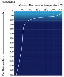
The Walker Circulations of the tropical Indian, Pacific, and Atlantic basins result in westerly surface winds in Northern Summer in the first basin and easterly winds in the second and third basins. As a result, the temperature structure of the three oceans display dramatic asymmetries. The equatorial Pacific and Atlantic both have cool surface temperatures in Northern Summer in the east, while cooler surface temperatures prevail only in the western Indian Ocean.[5] These changes in surface temperature reflect changes in the depth of the thermocline.[6]
Changes in the Walker Circulation with time occur in conjunction with changes in surface temperature. Some of these changes are forced externally, such as the seasonal shift of the Sun into the Northern Hemisphere in summer. Other changes appear to be the result of coupled ocean-atmosphere feedback in which, for example, easterly winds cause the sea surface temperature to fall in the east, enhancing the zonal heat contrast and hence intensifying easterly winds across the basin. These anomalous easterlies induce more equatorial upwelling and raise the thermocline in the east, amplifying the initial cooling by the southerlies. This coupled ocean-atmosphere feedback was originally proposed by Bjerknes. From an oceanographic point of view, the equatorial cold tongue is caused by easterly winds. Were the earth climate symmetric about the equator, cross-equatorial wind would vanish, and the cold tongue would be much weaker and have a very different zonal structure than is observed today.[7] The Walker cell is indirectly related to upwelling off the coasts of Peru and Ecuador. This brings nutrient-rich cold water to the surface, increasing fishing stocks.[8]
El Niño
The Walker circulation is caused by the pressure gradient force that results from a high pressure system over the eastern Pacific ocean, and a low pressure system over Indonesia. When the Walker circulation weakens or reverses, an El Niño results, causing the ocean surface to be warmer than average, as upwelling of cold water occurs less or not at all. An especially strong Walker circulation causes a La Niña, resulting in cooler ocean temperatures due to increased upwelling.
A scientific study published in May 2006 in the journal Nature indicates that the Walker circulation has been slowing since the mid-19th Century. The authors argue that global warming is a likely causative factor in the weakening of the wind pattern.[9] However, a new study from The Twentieth Century Reanalysis Project shows that the Walker circulation has not been slowing (or increasing) from 1871-2008.[10]
See also
References
- Walker Institute, University of Reading, UK. http://www.walker-institute.ac.uk/about/sir_gilbert.htm
- Walker, JM. Pen Portrait of Sir Gilbert Walker, CSI, MA, ScD, FRS. Weather 1997 (Volume 52, No.7, pages 217-220)
- Walker, G.T. and Bliss, E.W., 1930. World Weather IV, Memoirs of the Royal Meteorological Society, 3, (24), 81-95.
- Walker, G.T. and Bliss, E.W., 1937. World Weather VI, Memoirs of the Royal Meteorological Society, 4, (39), 119-139.
- Walker, G.T., 1923. Correlation in seasonal variations of weather, VIII. A preliminary study of world weather. Memoirs of the India Meteorological Department, 24, (4), 75-131.
- Walker, G.T., 1924. Correlation in seasonal variations of weather, IX. A further study of world weather. Memoirs of the India Meteorological Department, 24, (9),275-333. http://www.rmets.org/about/history/classics.php
- Katz, R.W. Sir Gilbert Walker and a Connection between El Nino and Statistics. Statistical Science, 17 (2002), 97-117. http://amath.colorado.edu/courses/4540/2004Spr/walkerss.pdf
- Climate research summary - Walker Circulation: a tropical atmospheric circulation slow-down Text and graphics from NOAA / Geophysical Fluid Dynamics Laboratory
- Slowdown in tropical Pacific flow pinned on climate change - press release from University Corporation for Atmospheric Research.
- Weakening of tropical Pacific atmospheric circulation due to anthropogenic forcing 4 May 2006 in Nature.
- Associated Press news story, 3 May 2006: "Global Warming Cited in Wind Shift"
- Tropical convective transport and the Walker circulation, 29 October 2012 in Atmospheric Chemistry and Physics
In-line citations
- 1 2 Rao, C. Hayavando, ed. (1915). The Indian Biographical Dictionary. Madras: Pillar & Co. p. 456. Retrieved 2010-03-20.
- ↑ AUTOCORRELATION FUNCTION
- ↑ AUTOREGRESSIVE MODELING
- ↑ Yule-Walker equations
- ↑ Bureau of Meteorology. "The Walker Circulation". Commonwealth of Australia. Retrieved 2014-07-01.
- ↑ Zelle, Hein, Gerrian Appledoorn, Gerritt Burgers, and Gert Jan Van Oldenborgh (March 2004). "Relationship Between Sea Surface Temperature and Thermocline Depth in the Eastern Equatorial Pacific". Journal of Physical Oceanography. American Meteorological Society. 34: 643. Bibcode:2004JPO....34..643Z. doi:10.1175/2523.1. Retrieved 2014-07-01.
- ↑ Ocean-atmosphere interaction in the making of the Walker circulation and equatorial cold tongue
- ↑ Jennings, S., Kaiser, M.J., Reynolds, J.D. (2001) "Marine Fisheries Ecology." Oxford: Blackwell Science Ltd. ISBN 0-632-05098-5
- ↑ A tropical atmospheric circulation slow-down
- ↑ The Twentieth Century Reanalysis Project. Quarterly Journal of the Royal Meteorological Society, 137: 1–28. doi:10.1002/qj.776, http://onlinelibrary.wiley.com/doi/10.1002/qj.776/abstract