Trilinear interpolation
Trilinear interpolation is a method of multivariate interpolation on a 3-dimensional regular grid. It approximates the value of an intermediate point  within the local axial rectangular prism linearly, using data on the lattice points. For an arbitrary, unstructured mesh (as used in finite element analysis), other methods of interpolation must be used; if all the mesh elements are tetrahedra (3D simplices), then barycentric coordinates provide a straightforward procedure.
Trilinear interpolation is frequently used in numerical analysis, data analysis, and computer graphics.
Compared to linear and bilinear interpolation
Trilinear interpolation is the extension of linear interpolation, which operates in spaces with dimension  , and bilinear interpolation, which operates with dimension
  , to dimension
  . The order of accuracy is 1 for all these interpolation schemes, and it requires
  adjacent pre-defined values surrounding the interpolation point. There are several ways to arrive at trilinear interpolation, it is equivalent to 3-dimensional tensor B-spline interpolation of order 1, and the trilinear interpolation operator is also a tensor product of 3 linear interpolation operators.
Method


On a periodic and cubic lattice, let  ,
,  , and
, and  be the differences between each of
  ,
,  ,
,  and the smaller coordinate related, that is:


where  indicates the lattice point below , and
  indicates the lattice point above and similarly for
 and
and  .
.
First we interpolate along (imagine we are pushing the front face of the cube to the back), giving:
![\ c_{00} = V[x_0,y_0, z_0] (1 - x_d) + V[x_1, y_0, z_0] x_d](../I/m/67340f3f50087d3667c69e7fd70b43a7.png)
![\ c_{01} = V[x_0,y_0, z_1] (1 - x_d) + V[x_1, y_0, z_1] x_d](../I/m/3e07ed88582df2be3c7b5669d777c8a9.png)
![\ c_{10} = V[x_0,y_1, z_0] (1 - x_d) + V[x_1, y_1, z_0] x_d](../I/m/e8d5fe4995d87bc1e6fc26164f2a3374.png)
![\ c_{11} = V[x_0,y_1, z_1] (1 - x_d) + V[x_1, y_1, z_1] x_d](../I/m/c1c3496f2d9be5048f1d40e5ddae02d0.png)
Where ![V[x_0,y_0, z_0]](../I/m/8f2f87a6ed7cbef256b3d3d82dbdc492.png) means the function value of
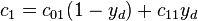
means the function value of  Then we interpolate these values (along , as we were pushing the top edge to the bottom), giving:

Finally we interpolate these values along (walking through a line):
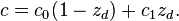
This gives us a predicted value for the point.
The result of trilinear interpolation is independent of the order of the interpolation steps along the three axes: any other order, for instance along , then along , and finally along , produces the same value.
The above operations can be visualized as follows: First we find the eight corners of a cube that surround our point of interest. These corners have the values C000, C100, C010, C110, C001, C101, C011, C111.
Next, we perform linear interpolation between C000 and C100 to find C00, C001 and C101 to find C01, C011 and C111 to find C11, C010 and C110 to find C10.
Now we do interpolation between C00 and C10 to find C0, C01 and C11 to find C1. Finally, we calculate the value C via linear interpolation of C0 and C1
In practice, a trilinear interpolation is identical to two bilinear interpolation combined with a linear interpolation:

See also
- Linear interpolation
- Bilinear interpolation
- Tricubic interpolation
- Radial interpolation
- Tetrahedral interpolation
External links
- pseudo-code from NASA, describes an iterative inverse trilinear interpolation (given the vertices and the value of C find Xd, Yd and Zd).
- Paul Bourke, Interpolation methods, 1999. Contains a very clever and simple method to find trilinear interpolation that is based on binary logic and can be extended to any dimension (Tetralinear, Pentalinear, ...).