Tanabe–Sugano diagram
Tanabe–Sugano diagrams are used in coordination chemistry to predict absorptions in the UV, visible and IR electromagnetic spectrum of coordination compounds. The results from a Tanabe–Sugano diagram analysis of a metal complex can also be compared to experimental spectroscopic data. They are qualitatively useful and can be used to approximate the value of 10Dq, the ligand field splitting energy. Tanabe–Sugano diagrams can be used for both high spin and low spin complexes, unlike Orgel diagrams, which apply only to high spin complexes. Tanabe–Sugano diagrams can also be used to predict the size of the ligand field necessary to cause high-spin to low-spin transitions.
In a Tanabe–Sugano diagram, the ground state is used as a constant reference, in contrast to Orgel diagrams. The energy of the ground state is taken to be zero for all field strengths, and the energies of all other terms and their components are plotted with respect to the ground term.
Background
Until Yukito Tanabe and Satoru Sugano published their paper "On the absorption spectra of complex ions", in 1954, little was known about the excited electronic states of complex metal ions. They used Hans Bethe's crystal field theory and Giulio Racah's linear combinations of Slater integrals,[1] now called Racah parameters, to explain the absorption spectra of octahedral complex ions in a more quantitative way than had been achieved previously.[2] Many spectroscopic experiments later, they estimated the values for two of Racah's parameters, B and C, for each d-electron configuration based on the trends in the absorption spectra of isoelectronic first-row transition metals. The plots of the energies calculated for the electronic states of each electron configuration are now known as Tanabe–Sugano diagrams.[3][4]
Parameters
The x-axis of a Tanabe–Sugano diagram is expressed in terms of the ligand field splitting parameter, Dq, or Δ, divided by the Racah parameter B. The y-axis is in terms of energy, E, also scaled by B. Three Racah parameters exist, A, B, and C, which describe various aspects of interelectronic repulsion. A is an average total interelectron repulsion. B and C correspond with individual d-electron repulsions. A is constant among d-electron configuration, and it is not necessary for calculating relative energies, hence its absence from Tanabe and Sugano's studies of complex ions. C is necessary only in certain cases. B is the most important of Racah's parameters in this case.[5] One line corresponds to each electronic state. The bending of certain lines is due to the mixing of terms with the same symmetry. Although electronic transitions are only "allowed" if the spin multiplicity remains the same (i.e. electrons do not change from spin up to spin down or vice versa when moving from one energy level to another), energy levels for "spin-forbidden" electronic states are included in the diagrams, which are also not included in Orgel diagrams.[6] Each state is given its symmetry label (e.g. A1g, T2g, etc.), but "g" and "u" subscripts are usually left off because it is understood that all the states are gerade. Labels for each state are usually written on the right side of the table, though for more complicated diagrams (e.g. d6) labels may be written in other locations for clarity. Term symbols (e.g. 3P, 1S, etc.) for a specific dn free ion are listed, in order of increasing energy, on the y-axis of the diagram. The relative order of energies is determined using Hund's rules. For an octahedral complex, the spherical, free ion term symbols split accordingly:[7]
| Term | Degeneracy | States in an octahedral field |
|---|---|---|
| S | 1 | A1g |
| P | 3 | T1g |
| D | 5 | Eg + T2g |
| F | 7 | A2g + T1g + T2g |
| G | 9 | A1g + Eg + T1g + T2g |
| H | 11 | Eg + T1g + T1g + T2g |
| I | 13 | A1g + A2g + Eg + T1g + T2g + T2g |
Certain Tanabe–Sugano diagrams (d4, d5, d6, and d7) also have a vertical line drawn at a specific Dq/B value, which corresponds with a discontinuity in the slopes of the excited states' energy levels. This pucker in the lines occurs when the spin pairing energy, P, is equal to the ligand field splitting energy, Dq. Complexes to the left of this line (lower Dq/B values) are high-spin, while complexes to the right (higher Dq/B values) are low-spin. There is no low-spin or high-spin designation for d2, d3, or d8.[8]
Tanabe-Sugano diagrams
The seven Tanabe–Sugano diagrams for octahedral complexes are shown below.[5][9][10]
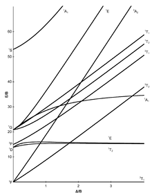 d2 electron configuration |
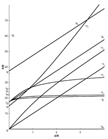 d3 electron configuration |
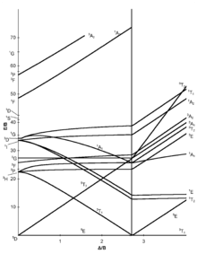 d4 electron configuration |
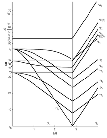 d5 electron configuration |
 d6 electron configuration |
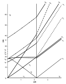 d7 electron configuration |
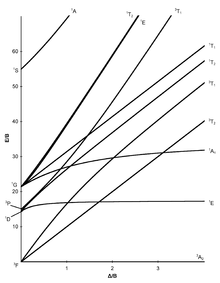 d8 electron configuration |
Unnecessary diagrams: d1, d9 and d10
d1
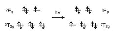
There is no electron repulsion in a d1 complex, and the single electron resides in the t2g orbital ground state. A d1 octahedral metal complex, such as [Ti(H2O)6]3+, shows a single absorption band in a UV-vis experiment.[5] The term symbol for d1 is 2D, which splits into the 2T2g and 2Eg states. The t2g orbital set holds the single electron and has a 2T2g state energy of -4Dq. When that electron is promoted to an eg orbital, it is excited to the 2Eg state energy, +6Dq. This is in accordance with the single absorption band in a UV-vis experiment. The prominent shoulder in this absorption band is due to a Jahn-Teller distortion which removes the degeneracy of the two 2Eg states. However, since these two transitions overlap in a UV-vis spectrum, this transition from 2T2g to 2Eg does not require a Tanabe–Sugano diagram.
d9
Similar to d1 metal complexes, d9 octahedral metal complexes have 2D spectral term. The transition is from the (t2g)6(eg)3 configuration (2Eg state) to the (t2g)5(eg)4 configuration (2T2g state). This could also be described as a positive "hole" that moves from the eg to the t2g orbital set. The sign of Dq is opposite that for d1, with a 2Eg ground state and a 2T2g excited state. Like the d1 case, d9 octahedral complexes do not require the Tanabe–Sugano diagram to predict their absorption spectra.
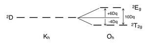 Splitting of 2D term in an octahedral crystal field |
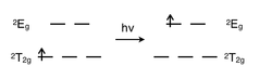 Electronic transition from ground state 2T2g to excited state 2Eg for a d1 electron configuration |
 Electronic transition from ground state to excited state for a d9 electron configuration |
d10
There are no d-d electron transitions in d10 metal complexes because the d orbitals are completely filled. Thus, UV-vis absorption bands are not observed and a Tanabe–Sugano diagram does not exist.
Diagrams for tetrahedral symmetry
Tetrahedral Tanabe–Sugano diagrams are generally not found in textbooks because the diagram for a dn tetrahedral will be similar to that for d(10-n) octahedral, remembering that ΔT for tetrahedral complexes is approximately 4/9 of ΔO for an octahedral complex. A consequence of the much smaller size of ΔT results in (almost) all tetrahedral complexes being high spin and therefore the change in the ground state term seen on the X-axis for octahedral d4-d7 diagrams is not required for interpreting spectra of tetrahedral complexes.
Advantages over Orgel diagrams
In Orgel diagrams, the magnitude of the splitting energy exerted by the ligands on d orbitals, as a free ion approach a ligand field, is compared to the electron-repulsion energy, which are both sufficient at providing the placement of electrons. However, if the ligand field splitting energy, 10Dq, is greater than the electron-repulsion energy, then Orgel diagrams fail in determining electron placement. In this case, Orgel diagrams are restricted to only high spin complexes.[6]
Tanabe–Sugano diagrams do not have this restriction, and can be applied to situations when 10Dq is significantly greater than electron repulsion. Thus, Tanabe–Sugano diagrams are utilized in determining electron placements for high spin and low spin metal complexes. However, they are limited in that they have only qualitative significance. Even so, Tanabe–Sugano diagrams are useful in interpreting UV-vis spectra and determining the value of 10Dq.[6]
Applications as a qualitative tool
In a centrosymmetric ligand field, such as in octahedral complexes of transition metals, the arrangement of electrons in the d-orbital is not only limited by electron repulsion energy, but it is also related to the splitting of the orbitals due to the ligand field. This leads to many more electron configuration states than is the case for the free ion. The relative energy of the repulsion energy and splitting energy defines the high-spin and low-spin states.
Considering both weak and strong ligand fields, a Tanabe–Sugano diagram shows the energy splitting of the spectral terms with the increase of the ligand field strength. It is possible for us to understand how the energy of the different configuration states is distributed at certain ligand strengths. The restriction of the spin selection rule makes it is even easier to predict the possible transitions and their relative intensity. Although they are qualitative, Tanabe–Sugano diagrams are very useful tools for analyzing UV-vis spectra: they are used to assign bands and calculate Dq values for ligand field splitting.[11][12]
Examples
Manganese(II) hexahydrate
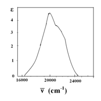
In the [Mn(H2O)6]2+ metal complex, manganese has an oxidation state of +2, thus it is a d5 ion. H2O is a weak field ligand (spectrum shown below), and according to the Tanabe–Sugano diagram for d5 ions, the ground state is 6A1. Note that there is no sextet spin multiplicity in any excited state, hence the transitions from this ground state are expected to be spin-forbidden and the band intensities should be low. From the spectra, only very low intensity bands are observed (low Molar absorptivity (ε) values on y-axis).[11]
Cobalt(II) hexahydrate
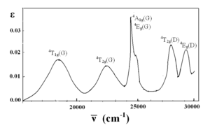
Another example is [Co(H2O)6]2+.[12] Note that the ligand is the same as the last example. Here the cobalt ion has the oxidation state of +2, and it is a d7 ion. From the high-spin (left) side of the d7 Tanabe–Sugano diagram, the ground state is 4T1(F), and the spin multiplicity is a quartet. The diagram shows that there are three quartet excited states: 4T2, 4A2, and 4T1(P). From the diagram one can predict that there are three spin-allowed transitions. However, the spectra of [Co(H2O)6]2+ does not show three distinct peaks that correspond to the three predicted excited states. Instead, the spectrum has a broad peak (spectrum shown below). Based on the T-S diagram, the lowest energy transition is 4T1 to 4T2, which is seen in the near IR and is not observed in the visible spectrum. The main peak is the energy transition 4T1(F) to 4T1(P), and the slightly higher energy transition (the shoulder) is predicted to be 4T1 to 4A2. The small energy difference leads to the overlap of the two peaks, which explains the broad peak observed in the visible spectrum.
Solving for B and ΔO
For the d2 complex [V(H2O)6]3+, two bands are observed with maxima at around 17,500 and 26,000 cm−1. The ratio of experimental band energies is E(ν2)/E(ν1) is 1.49. There are three possible transitions expected, which include: ν1: 3T1g→3T2g, ν2:3T1g→3T1g(P), and ν3: 3T1g→3A2g. There are three possible transitions, but only two are observed, so the unobserved transition must be determined.
| ΔO / B = | 10 | 20 | 30 | 40 |
|---|---|---|---|---|
| Height E(ν1)/B | 10 | 19 | 28 | 37 |
| Height E(ν2)/B | 23 | 33 | 42 | 52 |
| Height E(ν3)/B | 19 | 38 | 56 | 75 |
| Ratio E(ν3)/E(ν1) | 1.9 | 2.0 | 2.0 | 2.0 |
| Ratio E(ν2)/E(ν1) | 2.3 | 1.73 | 1.5 | 1.4 |
Fill in a chart like the one to the right by finding corresponding heights (E/B) of the symmetry states at certain values of ΔO / B. Then find the ratio of these values (E(ν2)/E(ν1) and E(ν3)/E(ν1)). Note that the ratio of E(ν3)/E(ν1) does not contain the calculated ratio for the experimental band energy, so we can determine that the 3T1g→3A2g band is unobserved. Use ratios for E(ν2)/E(ν1) and the values of ΔO / B to plot a line with E(ν2)/E(ν1) being the y-values and ΔO/B being the x-values. Using this line, it is possible to determine the value of ΔO / B for the experimental ratio. (ΔO / B = 31 for a chart ratio of 1.49 in this example).
Find on the T-S diagram where ΔO / B = 31 for 3T1g→3T2g and 3T1g→3T1g(P). For 3T2g, E(ν1) / B = 27 and for 3T1g(P), E(ν2) / B = 43.
The Racah parameter can be found by calculating B from both E(ν2) and E(ν1). For 3T1g(P), B = 26,000 cm−1/43 = 604 cm−1. For 3T2g, B = 17,500 cm−1/ 27 = 648 cm−1. From the average value of the Racah parameter, the ligand field splitting parameter can be found (ΔO). If ΔO / B = 31 and B = 625 cm−1, then ΔO = 19,375 cm−1.
See also
- Character tables
- Crystal field theory
- d electron count
- Hans Bethe
- Laporte rule
- Ligand field theory
- Molecular symmetry
- Orgel diagram
- Racah parameter
- Spin states (d electrons)
- Term symbol
References
- ↑ Racah, Giulio (1942). "Theory of complex spectra II". Physical Review. 62 (9–10): 438–462. Bibcode:1942PhRv...62..438R. doi:10.1103/PhysRev.62.438.
- ↑ Tanabe, Yukito; Sugano, Satoru (1954). "On the absorption spectra of complex ions I". Journal of the Physical Society of Japan. 9 (5): 753–766. doi:10.1143/JPSJ.9.753.
- ↑ Tanabe, Yukito; Sugano, Satoru (1954). "On the absorption spectra of complex ions II". Journal of the Physical Society of Japan. 9 (5): 766–779. doi:10.1143/JPSJ.9.766.
- ↑ Tanabe, Yukito; Sugano, Satoru (1956). "On the absorption spectra of complex ions III". Journal of the Physical Society of Japan. 11 (8): 864–877. doi:10.1143/JPSJ.11.864.
- 1 2 3 Atkins, Peter; Overton, Tina; Rourke, Jonathan; Weller, Mark; Armstrong, Fraser; Salvador, Paul; Hagerman, Michael; Spiro, Thomas; Stiefel, Edward (2006). Shriver & Atkins Inorganic Chemistry (4th ed.). New York: W.H. Freeman and Company. pp. 478–483. ISBN 0-7167-4878-9.
- 1 2 3 Douglas, Bodie; McDaniel, Darl; Alexander, John (1994). Concepts and Models of Inorganic Chemistry (3rd ed.). New York: John Wiley & Sons. pp. 442–458. ISBN 0-471-62978-2.
- ↑ Cotton, F. Albert; Wilkinson, Geoffrey; Gaus, Paul L. (1995). Basic Inorganic Chemistry (3rd ed.). New York: John Wiley & Sons. pp. 530–537. ISBN 0-471-50532-3.
- ↑ Harris, Daniel C.; Bertolucci, Michael D. (1978). Symmetry and Spectroscopy: An Introduction to Vibrational and Electronic Spectroscopy. New York: Dover Publications, Inc. pp. 403–409, 539. ISBN 978-0-486-66144-5.
- ↑ Lancashire, Robert John (4–10 June 1999), Interpretation of the spectra of first-row transition metal complexes (PDF), CONFCHEM, ACS Division of Chemical Education
- ↑ Lancashire, Robert John (25 September 2006). "Tanabe-Sugano diagrams via spreadsheets". Retrieved 29 November 2009.
- 1 2 Jørgensen, Chr Klixbüll; De Verdier, Carl-Henric; Glomset, John; Sörensen, Nils Andreas (1954). "Studies of absorption spectra IV: Some new transition group bands of low intensity". Acta Chem. Scand. 8 (9): 1502–1512. doi:10.3891/acta.chem.scand.08-1502.
- 1 2 Jørgensen, Chr Klixbüll; De Verdier, Carl-Henric; Glomset, John; Sörensen, Nils Andreas (1954). "Studies of absorption spectra III: Absoprtion Bands as Gaussian Error Curves". Acta Chem. Scand. 8 (9): 1495–1501. doi:10.3891/acta.chem.scand.08-1495.