Survival analysis
Survival analysis is a branch of statistics for analyzing the expected duration of time until one or more events happen, such as death in biological organisms and failure in mechanical systems. This topic is called reliability theory or reliability analysis in engineering, duration analysis or duration modelling in economics, and event history analysis in sociology. Survival analysis attempts to answer questions such as: what is the proportion of a population which will survive past a certain time? Of those that survive, at what rate will they die or fail? Can multiple causes of death or failure be taken into account? How do particular circumstances or characteristics increase or decrease the probability of survival?
To answer such questions, it is necessary to define "lifetime". In the case of biological survival, death is unambiguous, but for mechanical reliability, failure may not be well-defined, for there may well be mechanical systems in which failure is partial, a matter of degree, or not otherwise localized in time. Even in biological problems, some events (for example, heart attack or other organ failure) may have the same ambiguity. The theory outlined below assumes well-defined events at specific times; other cases may be better treated by models which explicitly account for ambiguous events.
More generally, survival analysis involves the modelling of time to event data; in this context, death or failure is considered an "event" in the survival analysis literature – traditionally only a single event occurs for each subject, after which the organism or mechanism is dead or broken. Recurring event or repeated event models relax that assumption. The study of recurring events is relevant in systems reliability, and in many areas of social sciences and medical research.
Introduction to survival analysis
Survival analysis is used in several ways:
- To describe the survival times of members of a group
- To compare the survival times of two or more groups
- To describe the effect of categorical or quantitative variables on survival
- Cox proportional hazards regression
- Parametric survival models
- Survival trees
- Survival random forests
Definitions of common terms in survival analysis
The following terms are commonly used in survival analyses.
- Event: Death, disease occurrence, disease recurrence, recovery, or other experience of interest
- Time: The time from the beginning of an observation period (such as surgery or beginning treatment) to (i) an event, or (ii) end of the study, or (iii) loss of contact or withdrawal from the study.
- Censoring / Censored observation: If a subject does not have an event during the observation time, they are described as censored. The subject is censored in the sense that nothing is observed or known about that subject after the time of censoring. A censored subject may or may not have an event after the end of observation time.
- Survival function S(t): The probability that a subject survives longer than time t.
Example: Acute Myelogenous Leukemia survival data
This example uses the Acute Myelogenous Leukemia survival data set "aml" from the "survival" package in R. The data set is from Miller (1997) [1] The question at the time was whether the standard course of chemotherapy should be extended ('maintained') for additional cycles.
The aml data set sorted by survival time is shown in the box.

- Time is indicated by the variable "time", which is the survival or censoring time
- Event (recurrence of aml cancer) is indicated by the variable "status". 0 = no event (censored), 1 = event (recurrence)
- Treatment group: the variable "x" indicates if maintenance chemotherapy was given
The last observation (11), at 161 weeks, is censored. Censoring indicates that the patient did not have an event (no recurrence of aml cancer). Another subject, observation 3, was censored at 13 weeks (indicated by status=0). This subject was only in the study for 13 weeks, and the aml cancer did not recur during those 13 weeks. It is possible that this patient was enrolled near the end of the study, so that they could only be observed for 13 weeks. It is also possible that the patient was enrolled early in the study, but was lost to follow up or withdrew from the study. The table shows that other subjects were censored at 16, 28, and 45 weeks (observations 17, 6, and 9 with status=0). The remaining subjects all experienced events (recurrence of aml cancer) while in the study. The question of interest is whether recurrence occurs later in maintained patients than in non-maintained patients.
Kaplan-Meier plot for the aml data
The Survival function S(t), is the probability that a subject survives longer than time t. S(t) is theoretically a smooth curve, but it is usually estimated using the Kaplan-Meier(KM) curve. The graph shows the KM plot for the aml data.

The KM plot is interpreted as follows.
- The x-axis is time, from zero (when observation began) to the last observed time point.
- The y axis is the proportion of subjects surviving. At time zero, 100% of the subjects are alive without an event.
- The solid line (similar to a staircase) shows the events.
- A vertical drop indicates an event. In the aml table shown above, two subjects had events at 5 weeks, two had events at 8 weeks, one had an event at 9 weeks, and so on. These events at 5 weeks, 8 weeks and so on are indicated by the vertical drops in the KM plot at those time points.
- At the far right end of the KM plot there is a tick mark at 161 weeks. The vertical tick mark indicates that a patient was censored at this time. In the aml data table five subjects were censored, at 13, 16, 28, 45 and 161 weeks. There are five tick marks in the KM plot, corresponding to these censored observations.
Life table for the aml data
A Life tables summarizes survival data in terms of the number of events and the proportion surviving at each event time point. The life table for the aml data, created using the R software, is shown.
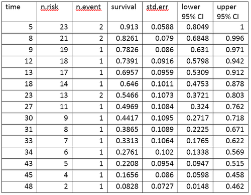
The life table summarizes the events and the proportion surviving at each event time point. The columns in the life table have the following interpretation.
- time gives the time points at which events occur.
- n.risk is the number of subjects at risk immediately before the time point, t. Being "at risk" means that the subject has not had an event before time t, and is not censored before or at time t.
- n.event is the number of subjects who have events at time t.
- survival is the proportion surviving, as determined using the Kaplan-Meier product-limit estimate.
- std.err is the standard error of the estimated survival. The standard error of the Kaplan-Meier product-limit estimate at time it is calculated using Greenwood’s formula, and depends on the number at risk (n.risk in the table), the number of deaths (n.event in the table) and the proportion surviving (survival in the table).
- lower 95% CI and upper 95% CI are the lower and upper 95% confidence bounds for the proportion surviving.
Log-rank test: Testing for differences in survival in the aml data
The logrank test compares the survival times of two or more groups. This example uses a logrank test for a difference in survival in the maintained versus non-maintained treatment groups in the aml data. The graph shows KM plots for the aml data broken out by treatment group, which is indicated by the variable "x" in the data.

The null hypothesis for a logrank test is that the groups have the same survival. The expected number of subjects surviving at each time point in each is adjusted for the number of subjects at risk in the groups at each event time. The logrank test determines if the observed number of events in each group is significantly different from the expected number. The formal test is based on a chi-squared statistic. When the log rank statistic is large, it is evidence for a different in the survival times between the groups. The log rank statistic has a chi-squared distribution with one degree of freedom, and the p-value is calculated using the chi-squared distribution.
The log rank test for difference in survival gives a p-value of p=0.0653, indicating that the treatment groups do not differ significantly in survival, although they approach significance. The sample size of 23 subjects is modest, so there is little power to detect differences between the treatment groups. The chi-squared test is based on asymptotic approximation, so the p-value should be regarded with caution for small sample sizes.
Cox proportional hazards (PH) regression analysis
Kaplan-Meier curves and logrank tests are most useful when the predictor variable is categorical (e.g., drug vs. placebo), or takes a small number of values (e.g., drug doses 0, 20, 50, and 100 mg/day) that can be treated as categorical. The logrank test and K-M curves don’t work easily with quantitative predictors such as gene expression, white blood count, or age. For quantitative predictor variables, an alternative method is Cox proportional hazards regression analysis. Cox PH models work also with categorical predictor variables, which are encoded as {0,1} indicator or dummy variables. The logrank test is a special case of a Cox PH analysis, and can be performed using Cox PH software.
Example: Cox proportional hazards regression analysis for melanoma
This example uses the melanoma data set from Dalgaard Chapter 12. [2]
Data are in the R package ISwR. The Cox proportional hazards regression using R gives the results shown in the box.
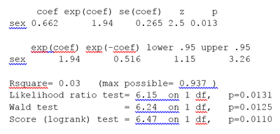
The Cox regression results are interpreted as follows.
- Sex is encoded as a numeric vector. 1: female, 2: male. The R summary for the cox model gives the hazard ratio (HR) for the second group relative to the first group, that is, male versus female.
- coef= 0.662 is the estimated logarithm of the hazard ratio for males versus females.
- exp(coef) = 1.94 = exp(0.662) The log of the hazard ratio (coef= 0.662) is transformed to the hazard ratio using exp(coef). The summary for the Cox model gives the hazard ratio for the second group relative to the first group, that is, male versus female. The estimated hazard ratio = 1.94 indicates that males have higher risk of death (lower survival rates) than females, in these data.
- se(coef) = 0.265 is the standard error of the log hazard ratio.
- z = 2.5 = coef/se(coef) = 0.662/0.265. Dividing the coef by its standard error gives the z score:
- p=0.013. The p-value corresponding to z=2.5 for sex is p=0.013, indicating that there is a significant difference in survival as a function of sex.
The summary output also gives upper and lower 95% confidence intervals for the hazard ratio, lower 95% bound = 1.15, upper 95% bound = 3.26.
Finally, the output gives p-values for three alternative tests for overall significance of the model:
- Likelihood ratio test= 6.15 on 1 df, p=0.0131
- Wald test = 6.24 on 1 df, p=0.0125
- Score (logrank) test = 6.47 on 1 df, p=0.0110
These three methods are asymptotically equivalent. For large enough N, they will give similar results. For small N, they may differ somewhat. The last row, "Score (logrank) test" is the result for the logrank test, with p=0.011, the same result as the logrank test, because the logrank test is a special case of a Cox PH regression. The Likelihood ratio test has better behavior for small sample sizes, so it is generally preferred.
Cox model using a covariate in the melanoma data
The Cox model extends the logrank test by allowing the inclusion of additional covariates. This example use the melanom data set where the predictor variables include a continuous covariate, the thickness of the tumor (variable name = “thick”)

In the histograms, the thickness values don’t look normally distributed. Regression models, including the Cox model, generally give more reliable results with normally-distributed variables. For this example use a log transform. The log of the thickness of the tumor looks to be more normally distributed, so the Cox models will use log thickness. The Cox PH analysis gives the results in the box.

The p-value for all three overall tests (likelihood, Wald, and score) are significant, indicating that the model is significant. The p-value for log(thick) is 6.9e-07, with a hazard ratio HR = exp(coef) = 2.18, indicating a strong relationship between the thickness of the tumor and increased risk of death.
By contrast, the p-value for sex is now p=0.088. The hazard ratio HR = exp(coef) = 1.58, with a 95% confidence interval of 0.934 to 2.68. Because the confidence interval for HR includes 1, these results indicate that sex makes a smaller contribution to the difference in the HR after controlling for the thickness of the tumor, and only trend toward significance. Examination of graphs of log(thickness) by sex and a t-test of log(thickness) by sex both indicate that there is a significant difference between men and women in the thickness of the tumor when they first see the clinician.
The Cox model assumes that the hazards are proportional. The proportional hazard assumption may be tested using the R function cox.zph(). A p-value is less than 0.05 indicates that the hazards are not proportional. For the melanoma data, p=0.222, indicating that the hazards are, at least approximately, proportional. Additional tests and graphs for examining a Cox model are described in the textbooks cited.
Extensions to Cox models
Cox models can be extended to deal with variations on the simple analysis.
- Stratification. The subjects can be divided into strata, where subjects within a stratum are expected to be relatively more similar to each other than to randomly chosen subjects from other strata. The regression parameters are assumed to be the same across the strata, but a different baseline hazard may exist for each stratum. Stratification is useful for analyses using matched subjects, for dealing with patient subsets, such as different clinics, and for dealing with violations of the proportional hazard assumption.
- Time-varying covariates. Some variables, such as gender and treatment group, generally stay the same in a clinical trial. Other clinical variables, such as serum protein levels or dose of concomitant medications may change over the course of a study. Cox models may be extended for such time-varying covariates.
Tree-structured survival models
The Cox PH regression model is a linear model. It is similar to linear regression and logistic regression. Specifically, these methods assume that a single line, curve, plane, or surface is sufficient to separate groups (alive, dead) or to estimate a quantitative response (survival time).
In some cases alternative partitions give more accurate classification or quantitative estimates. One set of alternative methods are tree-structured survival models, including survival random forests. Tree-structured survival models may give more accurate predictions than Cox models. Examining both types of models for a given data set is a reasonable strategy.
Example survival tree analysis
This example of a survival tree analysis uses the R package "rpart". The example is based on 146 stage C prostate cancer patients in the data set stagec in rpart. Rpart and the stagec example are described in the PDF document "An Introduction to Recursive Partitioning Using the RPART Routines". Terry M. Therneau, Elizabeth J. Atkinson, Mayo Foundation. September 3, 1997.
The variables in stagec are:
- pgtime time to progression, or last follow-up free of progression
- pgstat status at last follow-up (1=progressed, 0=censored)
- age age at diagnosis
- eet early endocrine therapy (1=no, 0=yes)
- ploidy diploid/tetraploid/aneuploid DNA pattern
- g2 % of cells in G2 phase
- grade tumor grade (1-4)
- gleason Gleason grade (3-10)
The survival tree produced by the analysis is shown in the figure.
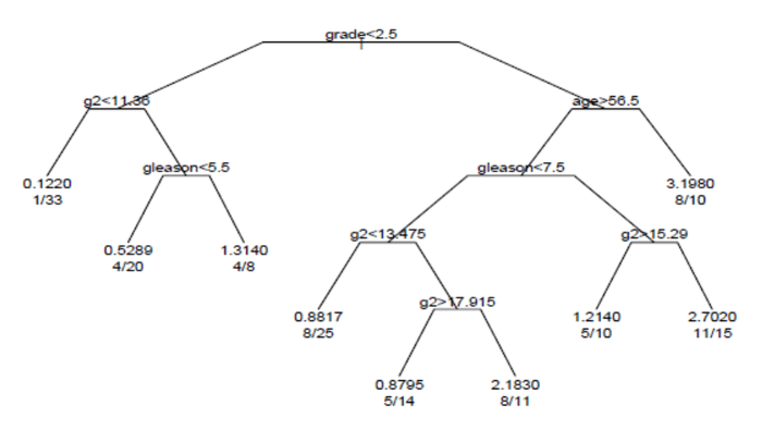
Each branch in the tree indicates a split on the value of a variable. For example, the root of the tree splits subjects with grade < 2.5 versus subjects with grade 2.5 or greater. The terminal nodes indicate the number of subjects in the node, the number of subjects who have events, and the relative event rate compared to the root. In the node on the far left, the values 1/33 indicate that 1 of the 33 subjects in the node had an event, and that the relative event rate is 0.122. In the node on the far right bottom, the values 11/15 indicate that 11 of 15 subjects in the node had an event, and the relative event rate is 2.7.
Survival random forests
An alternative to building a single survival tree is to build many survival trees, where each tree is constructed using a sample of the data, and average the trees to predict survival. This is the method underlying the survival random forest models. Survival random forest analysis is available in the R package "randomForestSRC".
The randomForestSRC package includes an example survival random forest analysis using the data set pbc. This data is from the Mayo Clinic Primary Biliary Cirrhosis (PBC) trial of the liver conducted between 1974 and 1984. In the example, the random forest survival model gives more accurate predictions of survival than the Cox PH model. The prediction errors are estimated by bootstrap re-sampling.
General formulation
Survival function
The object of primary interest is the survival function, conventionally denoted S, which is defined as

where t is some time, T is a random variable denoting the time of death, and "Pr" stands for probability. That is, the survival function is the probability that the time of death is later than some specified time t. The survival function is also called the survivor function or survivorship function in problems of biological survival, and the reliability function in mechanical survival problems. In the latter case, the reliability function is denoted R(t).
Usually one assumes S(0) = 1, although it could be less than 1 if there is the possibility of immediate death or failure.
The survival function must be non-increasing: S(u) ≤ S(t) if u ≥ t. This property follows directly because T>u implies T>t. This reflects the notion that survival to a later age is only possible if all younger ages are attained. Given this property, the lifetime distribution function and event density (F and f below) are well-defined.
The survival function is usually assumed to approach zero as age increases without bound, i.e., S(t) → 0 as t → ∞, although the limit could be greater than zero if eternal life is possible. For instance, we could apply survival analysis to a mixture of stable and unstable carbon isotopes; unstable isotopes would decay sooner or later, but the stable isotopes would last indefinitely.
Lifetime distribution function and event density
Related quantities are defined in terms of the survival function.
The lifetime distribution function, conventionally denoted F, is defined as the complement of the survival function,

If F is differentiable then the derivative, which is the density function of the lifetime distribution, is conventionally denoted f,

The function f is sometimes called the event density; it is the rate of death or failure events per unit time.
The survival function can be expressed in terms of probability distribution and probability density functions

Similarly, a survival event density function can be defined as
![s(t)=S'(t)={\frac {d}{dt}}S(t)={\frac {d}{dt}}\int _{t}^{{\infty }}f(u)\,du={\frac {d}{dt}}[1-F(t)]=-f(t).](../I/m/aef0f76f4ba2197d146ecf3b9c3d50d7eb4fdb16.svg)
The survival event density function in other fields, such as Statistical Physics is known as the first passage time density.
Hazard function and cumulative hazard function
The hazard function, conventionally denoted , is defined as the event rate at time t conditional on survival until time t or later (that is, T ≥ t). Suppose that an item has survived for a time t and we desire the probability that it will not survive for an additional time dt. That is, consider P{X (t,t + dt)|X > t}


Force of mortality is a synonym of hazard function which is used particularly in demography and actuarial science, where it is denoted by . The term hazard rate is another synonym.

The force of mortality of the survival function is defined as

The force of mortality is also called the force of failure. is the probability density function of the distribution.
In actuarial science, the hazard rate is the rate of death for lives aged x. For a life aged x, the force of mortality t years later is the force of mortality for a (x + t)–year old. The hazard rate is also called the failure rate. Hazard rate and failure rate are names used in reliability theory.
Any function is a hazard function if and only if it satisfies the following properties:
- ,
- .


In fact, the hazard rate is usually more informative about the underlying mechanism of failure than the other representatives of a lifetime distribution.
The hazard function must be non-negative, λ(t) ≥ 0, and its integral over must be infinite, but is not otherwise constrained; it may be increasing or decreasing, non-monotonic, or discontinuous. An example is the bathtub curve hazard function, which is large for small values of t, decreasing to some minimum, and thereafter increasing again; this can model the property of some mechanical systems to either fail soon after operation, or much later, as the system ages.
![[0,\infty ]](../I/m/52088d5605716e18068a460dec118214954a68e9.svg)
The hazard function can alternatively be represented in terms of the cumulative hazard function, conventionally denoted :


so transposing signs and exponentiating

or differentiating (with the chain rule)

The name "cumulative hazard function" is derived from the fact that

which is the "accumulation" of the hazard over time.
From the definition of , we see that it increases without bound as t tends to infinity (assuming that S(t) tends to zero). This implies that must not decrease too quickly, since, by definition, the cumulative hazard has to diverge. For example, is not the hazard function of any survival distribution, because its integral converges to 1.


Quantities derived from the survival distribution
Future lifetime at a given time is the time remaining until death, given survival to age . Thus, it is in the present notation. The expected future lifetime is the expected value of future lifetime. The probability of death at or before age , given survival until age , is just


Therefore, the probability density of future lifetime is

and the expected future lifetime is

where the second expression is obtained using integration by parts.
For , that is, at birth, this reduces to the expected lifetime.

In reliability problems, the expected lifetime is called the mean time to failure, and the expected future lifetime is called the mean residual lifetime.
As the probability of an individual surviving until age t or later is S(t), by definition, the expected number of survivors at age t out of an initial population of n newborns is n × S(t), assuming the same survival function for all individuals. Thus the expected proportion of survivors is S(t). If the survival of different individuals is independent, the number of survivors at age t has a binomial distribution with parameters n and S(t), and the variance of the proportion of survivors is S(t) × (1-S(t))/n.
The age at which a specified proportion of survivors remain can be found by solving the equation S(t) = q for t, where q is the quantile in question. Typically one is interested in the median lifetime, for which q = 1/2, or other quantiles such as q = 0.90 or q = 0.99.
One can also make more complex inferences from the survival distribution. In mechanical reliability problems, one can bring cost (or, more generally, utility) into consideration, and thus solve problems concerning repair or replacement. This leads to the study of renewal theory and reliability theory of ageing and longevity.
Censoring
Censoring is a form of missing data problem which is common in survival analysis. Ideally, both the birth and death dates of a subject are known, in which case the lifetime is known.
If it is known only that the date of death is after some date, this is called right censoring. Right censoring will occur for those subjects whose birth date is known but who are still alive when they are lost to follow-up or when the study ends.
If a subject's lifetime is known to be less than a certain duration, the lifetime is said to be left-censored. Left censoring is usually applied when subjects in a study already have exhibited the event in question at the start of the study but information about when they first reached the event is unclear.[3]
It may also happen that subjects with a lifetime less than some threshold may not be observed at all: this is called truncation. Note that truncation is different from left censoring, since for a left censored datum, we know the subject exists, but for a truncated datum, we may be completely unaware of the subject. Truncation is also common. In a so-called delayed entry study, subjects are not observed at all until they have reached a certain age. For example, people may not be observed until they have reached the age to enter school. Any deceased subjects in the pre-school age group would be unknown. Left-truncated data are common in actuarial work for life insurance and pensions.[4]
We generally encounter right-censored data. Left-censored data can occur when a person's survival time becomes incomplete on the left side of the follow-up period for the person. For example, in a epidemiological example, we may monitor a patient for a infectious disorder starting from the time when he or she is tested positive for the infection. Although we may know the right-hand side of the duration of interest, we may never know the exact time of exposure to the infectious agent.[5]
Fitting parameters to data
Survival models can be usefully viewed as ordinary regression models in which the response variable is time. However, computing the likelihood function (needed for fitting parameters or making other kinds of inferences) is complicated by the censoring. The likelihood function for a survival model, in the presence of censored data, is formulated as follows. By definition the likelihood function is the conditional probability of the data given the parameters of the model. It is customary to assume that the data are independent given the parameters. Then the likelihood function is the product of the likelihood of each datum. It is convenient to partition the data into four categories: uncensored, left censored, right censored, and interval censored. These are denoted "unc.", "l.c.", "r.c.", and "i.c." in the equation below.

For uncensored data, with equal to the age at death, we have


For left-censored data, such that the age at death is known to be less than , we have

For right-censored data, such that the age at death is known to be greater than , we have

For an interval censored datum, such that the age at death is known to be less than and greater than , we have


An important application where interval-censored data arises is current status data, where an event is known not to have occurred before an observation time and to have occurred before the next observation time.
Non-parametric estimation
The Kaplan-Meier estimator can be used to estimate the survival function. The Nelson–Aalen estimator can be used to provide a non-parametric estimate of the cumulative hazard rate function.
Computer software for survival analysis
The UCLA website http://www.ats.ucla.edu/stat/ has numerous examples of statistical analyses using SAS, R, SPSS and STATA, including survival analyses.
The textbook by Kleinbaum [6] has examples of survival analyses using SAS, R, and other packages. The textbooks by Brostrom [7] by Dalgaard [2] and by Tableman and Kim [8] give examples of survival analyses using R (or using S, and which run in R).
Survival analysis in R
The code below performs the analyses on this Wikipedia page.
Analyses using the R package "survival"
The examples above use the R package "survival", except for the tree analyses described below.
# Install and load the survival package

install.packages("survival")
library(survival)

# sort the aml data by time
aml=aml[order(aml$time),]

aml
# Create graph of length of time that each subject was in the study
with(aml, plot(time, type="h"))

# Create the life table survival object for aml
aml.survfit = survfit(Surv(time, status == 1) ~ 1, data=aml)

# Plot the Kaplan-Meier curve for aml. Don't print the confidence interval.
plot(aml.survfit, xlab = "Time (weeks)", ylab="Proportion surviving", conf.int=FALSE, main="Survival in AML")

# Create the life table for the aml data
# The functions survfit() and Surv() create a life table survival object.
# The summary() function displays the life table
# The life table object is passed to the plot() function to create the KM plot.
aml.survfit = survfit(Surv(time, status == 1) ~ 1, data=aml)

summary(aml.survfit)

# Kaplan-Meier curve for aml with the confidence bounds.
# By default, R includes the confidence interval.
plot(aml.survfit, xlab = "Time", ylab="Proportion surviving")

# Create aml life tables and KM plots broken out by treatment (x,  "Maintained" vs. "Not maintained")
surv.by.aml.rx = survfit(Surv(time, status == 1) ~ x, data = aml)

summary(surv.by.aml.rx)

# Plot KM
plot(surv.by.aml.rx, xlab = "Time", ylab="Survival",col=c("black", "red"), lty = 1:2, main="Kaplan-Meier Survival vs. Maintenance in AML")

# Add legend
legend(100, .6, c("Maintained", "Not maintained"), lty = 1:2, col=c("black", "red"))

# Perform the log rank test using the R function survdiff().

surv.diff.aml= survdiff(Surv(time, status == 1) ~ x, data=aml)

surv.diff.aml

# Cox Proportional Hazards regression
# melanoma data set from ISwR package, described in Dalgaard Chapter 12.
# install the ISwR package and load the library into R.
# The ISwR package currently only appears to be available for older versions of R

install.packages("ISwR")

library(ISwR)

help(melanom) # description of the melanoma data

# The log rank test is a special case of the cox proportional hazard regression analysis.
# The same analysis can be performed using the R function coxph().
# melanoma example using a log-rank test.
surv.diff.sex = survdiff(Surv(days, status == 1) ~ sex, data = melanom)

surv.diff.sex

# melanoma analysis using Cox proportional hazards regression
coxph.sex = coxph(Surv(days, status == 1) ~ sex, data = melanom)

summary(coxph.sex)

# melanoma Cox analysis including covariate ulcer thickness

# Plot the thickness values and log(thickness)
hist(melanom$thick)

hist(log(melanom$thick))

# The Cox PH analysis of melanoma data including covariate log(thick)

coxph.sex.thick = coxph(Surv(days, status == 1) ~ sex + log(thick), data = melanom)

summary(coxph.sex.thick)

# Examine thickness by sex
boxplot(log(melanom$thick) ~ melanom$sex)

t.test(log(melanom$thick) ~ melanom$sex)

# Test of proportional hazards assumption
coxph.sex = coxph(Surv(days, status == 1) ~ sex, data = melanom)

cox.zph(coxph.sex)
Survival tree analysis using the rpart package
Rpart and the example are described in the PDF document "An Introduction to Recursive Partitioning Using the RPART Routines". Terry M. Therneau, Elizabeth J. Atkinson, Mayo Foundation. September 3, 1997.
install.packages("rpart")
library(rpart)

head(stagec)

# Pass a survival object from Surv() to the function rpart() to perform the analysis.
fit <- rpart(Surv(pgtime, pgstat) ~ age + eet + g2 + grade + gleason + ploidy, data=stagec)

# plot the resulting tree

plot(fit, uniform=T, branch=.4, compress=T)
text(fit, use.n=T)
# The print() function provides details of the tree not shown above
print(fit)
Survival random forest models using the randomForestSRC package
Note that the R package randomSurvivalForest has been replaced by the package randomForestSRC, "Random Forests for Survival, Regression and Classification". See the randomForestSRC package for documentation on running the example.
install.packages("randomForestSRC")
library("randomForestSRC")

# The pec example uses the R packages survival and pec.
library(survival)
install.packages("pec")
library(pec)

# Create Kaplan-Meier plot by treatment group
pbc.surv.by.treatment = survfit(Surv(days, status) ~ treatment, data = pbc)
plot(pbc.surv.by.treatment, xlab = "Days", ylab="Survival",col=c("black", "red"), lty = 1:2, main="Kaplan-Meier Survival vs. Treatment in PBC")
legend(100, .6, c("Rx1", "Rx2"), lty = 1:2, col=c("black", "red"))
Distributions used in survival analysis
- Exponential distribution
- Weibull distribution
- Log-logistic distribution
- Gamma distribution
- Exponential-logarithmic distribution
See also
References
- ↑ Miller, Rupert G. (1997), Survival analysis, John Wiley & Sons, ISBN 0-471-25218-2
- 1 2 Dalgaard, Peter (2008), Introductory Statistics with R (Second ed.), Springer, ISBN 978-0387790534
- ↑ "Censoring, Left and Right." International Encyclopedia of the Social Sciences, edited by William A. Darity, Jr., 2nd ed., vol. 1, Macmillan Reference USA, 2008, pp. 473-474. libraries.state.ma.us/login?gwurl=http://ic.galegroup.com/ic/uhic/ReferenceDetailsPage/ReferenceDetailsWindow?disableHighlighting=false&displayGroupName=Reference&currPage=&scanId=&query=&prodId=UHIC&search_within_results=&p=UHIC%3AWHIC&mode=view&catId=&limiter=&display-query=&displayGroups=&contentModules=&action=e&sortBy=&documentId=GALE%7CCX3045300295&windowstate=normal&activityType=&failOverType=&commentary=&source=Bookmark&u=mlin_w_amhercol&jsid=0938fef854cc86b83b5fe8a2c4bcb54b. Accessed 6 Nov. 2016.
- ↑ Richards, S. J. (2012). "A handbook of parametric survival models for actuarial use". Scandinavian Actuarial Journal. 2012 (4): 233–257. doi:10.1080/03461238.2010.506688.
- ↑ Singh, R.; Mukhopadhyay, K. (2011). "Survival analysis in clinical trials: Basics and must know areas". Perspect Clin Res. 2 (4): 145–148. doi:10.4103/2229-3485.86872.
- ↑ Kleinbaum, David G.; Klein, Mitchel (2012), Survival analysis: A Self-learning text (Third ed.), Springer, ISBN 978-1441966452
- ↑ Brostrom, Göran (2012), Event History Analysis with R (First ed.), Chapman & Hall/CRC, ISBN 978-1439831649
- ↑ Tableman, Mara; Kim, Jong Sung (2003), Survival Analysis Using S (First ed.), Chapman and Hall/CRC, ISBN 978-1584884088
Further reading
- Collett, David (2003). Modelling Survival Data in Medical Research (Second ed.). Boca Raton: Chapman & Hall/CRC. ISBN 1584883251.
- Elandt-Johnson, Regina; Johnson, Norman (1999). Survival Models and Data Analysis. New York: John Wiley & Sons. ISBN 0471349925.
- Kalbfleisch, J. D.; Prentice, Ross L. (2002). The statistical analysis of failure time data. New York: John Wiley & Sons. ISBN 047136357X.
- Lawless, Jerald F. (2003). Statistical Models and Methods for Lifetime Data (2nd ed.). Hoboken: John Wiley and Sons. ISBN 0471372153.
- Rausand, M.; Hoyland, A. (2004). System Reliability Theory: Models, Statistical Methods, and Applications. Hoboken: John Wiley & Sons. ISBN 047147133X.
External links
- Therneau, Terry. "A Package for Survival Analysis in S". via Dr. Therneau's page on the Mayo Clinic website
- "Engineering Statistics Handbook". NIST/SEMATEK.
- SOCR, Survival analysis applet and interactive learning activity.
- Survival/Failure Time Analysis @ Statistics' Textbook Page
- Survival Analysis in R
- Lifelines, a Python package for survival analysis
- Survival Analysis in NAG Fortran Library
| |||||||||||||||||||||||||||||||||||||||||||||
| |||||||||||||||||||||||||||||||||||||||||||||
| |||||||||||||||||||||||||||||||||||||||||||||
| |||||||||||||||||||||||||||||||||||||||||||||
| |||||||||||||||||||||||||||||||||||||||||||||
| |||||||||||||||||||||||||||||||||||||||||||||
| |||||||||||||||||||||||||||||||||||||||||||||