Stokes' theorem
| Part of a series of articles about | ||||||
| Calculus | ||||||
|---|---|---|---|---|---|---|
|
||||||
|
Specialized |
||||||
In vector calculus, and more generally differential geometry, Stokes' theorem (also called the generalized Stokes' theorem) is a statement about the integration of differential forms on manifolds, which both simplifies and generalizes several theorems from vector calculus. Stokes' theorem says that the integral of a differential form ω over the boundary of some orientable manifold Ω is equal to the integral of its exterior derivative dω over the whole of Ω, i.e.,

This modern form of Stokes' theorem is a vast generalization of a classical result. Lord Kelvin communicated it to George Stokes in a letter dated July 2, 1850.[1][2][3] Stokes set the theorem as a question on the 1854 Smith's Prize exam, which led to the result bearing his name, even though it was actually first published by Hermann Hankel in 1861.[3][4] This classical Kelvin–Stokes theorem relates the surface integral of the curl of a vector field F over a surface Σ in Euclidean three-space to the line integral of the vector field over its boundary ∂Σ:

This classical statement, along with the classical divergence theorem, the fundamental theorem of calculus, and Green's theorem are simply special cases of the general formulation stated above.
Introduction
The fundamental theorem of calculus states that the integral of a function f over the interval [a, b] can be calculated by finding an antiderivative F of f:

Stokes' theorem is a vast generalization of this theorem in the following sense.
- By the choice of F, dF/dx = f(x). In the parlance of differential forms, this is saying that f(x) dx is the exterior derivative of the 0-form, i.e. function, F: in other words, that dF = f dx. The general Stokes theorem applies to higher differential forms ω instead of just 0-forms such as F.
- A closed interval [a, b] is a simple example of a one-dimensional manifold with boundary. Its boundary is the set consisting of the two points a and b. Integrating f over the interval may be generalized to integrating forms on a higher-dimensional manifold. Two technical conditions are needed: the manifold has to be orientable, and the form has to be compactly supported in order to give a well-defined integral.
- The two points a and b form the boundary of the closed interval. More generally, Stokes' theorem applies to oriented manifolds M with boundary. The boundary ∂M of M is itself a manifold and inherits a natural orientation from that of the manifold. For example, the natural orientation of the interval gives an orientation of the two boundary points. Intuitively, a inherits the opposite orientation as b, as they are at opposite ends of the interval. So, "integrating" F over two boundary points a, b is taking the difference F(b) − F(a).
In even simpler terms, one can consider that points can be thought of as the boundaries of curves, that is as 0-dimensional boundaries of 1-dimensional manifolds. So, just as one can find the value of an integral (f dx = dF) over a 1-dimensional manifold ([a, b]) by considering the anti-derivative (F) at the 0-dimensional boundaries ({a, b}), one can generalize the fundamental theorem of calculus, with a few additional caveats, to deal with the value of integrals (dω) over n-dimensional manifolds (Ω) by considering the antiderivative (ω) at the (n − 1)-dimensional boundaries (∂Ω) of the manifold.
So the fundamental theorem reads:
![{\displaystyle \int _{[a,b]}f(x)\,dx=\int _{[a,b]}dF=\int _{\{a\}^{-}\cup \{b\}^{+}}F=F(b)-F(a)\,.}](../I/m/23cc3c08d9bb869053461d0eb1e277cc309f09c9.svg)
Formulation for smooth manifolds with boundary
Let Ω be an oriented smooth manifold with boundary of dimension n and let α be a smooth n-differential form that is compactly supported on Ω. First, suppose that α is compactly supported in the domain of a single, oriented coordinate chart {U, φ}. In this case, we define the integral of α over Ω as

i.e., via the pullback of α to Rn.
More generally, the integral of α over Ω is defined as follows: Let {ψi} be a partition of unity associated with a locally finite cover {Ui, φi} of (consistently oriented) coordinate charts, then define the integral

where each term in the sum is evaluated by pulling back to Rn as described above. This quantity is well-defined; that is, it does not depend on the choice of the coordinate charts, nor the partition of unity.
Stokes' theorem reads: If ω is an (n − 1)-form with compact support on Ω, and ∂Ω denotes the boundary of Ω with its induced orientation, then

Here d is the exterior derivative, which is defined using the manifold structure only. On the right-hand side, a circle is sometimes used within the integral sign to stress the fact that the (n − 1)-manifold ∂Ω is closed.[note 1] The right-hand side of the equation is often used to formulate integral laws; the left-hand side then leads to equivalent differential formulations (see below).
The theorem is often used in situations where Ω is an embedded oriented submanifold of some bigger manifold on which the form ω is defined.
Topological preliminaries; integration over chains
Let M be a smooth manifold. A (smooth) singular k-simplex in M is defined as a smooth map from the standard simplex in Rk to M. The group Ck(M, Z) of singular k-chains on M is defined to be the free abelian group on the set of singular k-simplices in M. These groups, together with the boundary map, ∂, define a chain complex. The corresponding homology (resp. cohomology) group is isomorphic to the usual singular homology group Hk(M, Z) (resp. the singular cohomology group Hk(M, Z)), defined using continuous rather than smooth simplices in M.
On the other hand, the differential forms, with exterior derivative, d, as the connecting map, form a cochain complex, which defines the de Rham cohomology groups Hk
dR(M, R).
Differential k-forms can be integrated over a k-simplex in a natural way, by pulling back to Rk. Extending by linearity allows one to integrate over chains. This gives a linear map from the space of k-forms to the kth group of singular cochains, Ck(M, Z), the linear functionals on Ck(M, Z). In other words, a k-form ω defines a functional

on the k-chains. Stokes' theorem says that this is a chain map from de Rham cohomology to singular cohomology with real coefficients; the exterior derivative, d, behaves like the dual of ∂ on forms. This gives a homomorphism from de Rham cohomology to singular cohomology. On the level of forms, this means:
- closed forms, i.e., dω = 0, have zero integral over boundaries, i.e. over manifolds that can be written as ∂∑c Mc, and
- exact forms, i.e., ω = dσ, have zero integral over cycles, i.e. if the boundaries sum up to the empty set: ∑c Mc = ∅.
De Rham's theorem shows that this homomorphism is in fact an isomorphism. So the converse to 1 and 2 above hold true. In other words, if {ci} are cycles generating the kth homology group, then for any corresponding real numbers, {ai}, there exist a closed form, ω, such that

and this form is unique up to exact forms.
Underlying principle

To simplify these topological arguments, it is worthwhile to examine the underlying principle by considering an example for d = 2 dimensions. The essential idea can be understood by the diagram on the left, which shows that, in an oriented tiling of a manifold, the interior paths are traversed in opposite directions; their contributions to the path integral thus cancel each other pairwise. As a consequence, only the contribution from the boundary remains. It thus suffices to prove Stokes' theorem for sufficiently fine tilings (or, equivalently, simplices), which usually is not difficult.
Generalization to rough sets

The formulation above, in which Ω is a smooth manifold with boundary, does not suffice in many applications. For example, if the domain of integration is defined as the plane region between two x-coordinates and the graphs of two functions, it will often happen that the domain has corners. In such a case, the corner points mean that Ω is not a smooth manifold with boundary, and so the statement of Stokes' theorem given above does not apply. Nevertheless, it is possible to check that the conclusion of Stokes' theorem is still true. This is because Ω and its boundary are well-behaved away from a small set of points (a measure zero set).
A version of Stokes' theorem that extends to rough domains was proved by Whitney.[5] Assume that D is a connected bounded open subset of of Rn. Call D a standard domain if it satisfies the following property: There exists a subset P of ∂D, open in ∂D, whose complement in ∂D has Hausdorff (n − 1)-measure zero; and such that every point of P has a generalized normal vector. This is a vector v(x) such that, if a coordinate system is chosen so that v(x) is the first basis vector, then, in an open neighborhood around x, there exists a smooth function f(x2, …, xn) such that P is the graph { x1 = f(x2, …, xn) } and D is the region { x1 < f(x2, …, xn) }. Whitney remarks that the boundary of a standard domain is the union of a set of zero Hausdorff (n − 1)-measure and a finite or countable union of smooth (n − 1)-manifolds, each of which has the domain on only one side. He then proves that if D is a standard domain in Rn, ω is an (n − 1)-form which is defined, continuous, and bounded on D ∪ P, smooth on D, integrable on P, and such that dω is integrable on D, then Stokes' theorem holds, that is,

The study of measure-theoretic properties of rough sets leads to geometric measure theory. Even more general versions of Stokes' theorem have been proved by Federer and by Harrison.[6]
Special cases
The general form of the Stokes theorem using differential forms is more powerful and easier to use than the special cases. The traditional versions can be formulated using Cartesian coordinates without the machinery of differential geometry, and thus are more accessible. Further, they are older and their names are more familiar as a result. The traditional forms are often considered more convenient by practicing scientists and engineers but the non-naturalness of the traditional formulation becomes apparent when using other coordinate systems, even familiar ones like spherical or cylindrical coordinates. There is potential for confusion in the way names are applied, and the use of dual formulations.
Kelvin–Stokes theorem
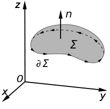
This is a (dualized) 1 + 1-dimensional case, for a 1-form (dualized because it is a statement about vector fields). This special case is often just referred to as the Stokes' theorem in many introductory university vector calculus courses and as used in physics and engineering. It is also sometimes known as the curl theorem.
The classical Kelvin–Stokes theorem:

which relates the surface integral of the curl of a vector field over a surface Σ in Euclidean three-space to the line integral of the vector field over its boundary, is a special case of the general Stokes theorem (with n = 2) once we identify a vector field with a 1-form using the metric on Euclidean 3-space. The curve of the line integral, ∂Σ, must have positive orientation, meaning that dr points counterclockwise when the surface normal, dΣ, points toward the viewer, following the right-hand rule.
One consequence of the Kelvin–Stokes theorem is that the field lines of a vector field with zero curl cannot be closed contours. The formula can be rewritten as:
![{\displaystyle {\begin{aligned}\iint _{\Sigma }&{\Bigg (}\left({\frac {\partial R}{\partial y}}-{\frac {\partial Q}{\partial z}}\right)\,dy\,dz+\left({\frac {\partial P}{\partial z}}-{\frac {\partial R}{\partial x}}\right)\,dz\,dx+\left({\frac {\partial Q}{\partial x}}-{\frac {\partial P}{\partial y}}\right)\,dx\,dy{\Bigg )}\\[8px]&=\oint _{\partial \Sigma }{\Big (}P\,dx+Q\,dy+R\,dz{\Big )}\,,\end{aligned}}}](../I/m/89dbd321d685d332affbea97cda0374bc71d1333.svg)
where P, Q and R are the components of F.
These variants are rarely used:
![{\displaystyle {\begin{aligned}&\int _{\Sigma }{\Big (}g\left(\nabla \times \mathbf {F} \right)+\left(\nabla g\right)\times \mathbf {F} {\Big )}\cdot d{\boldsymbol {\Sigma }}=\oint _{\partial \Sigma }g\mathbf {F} \cdot d\mathbf {r} \,,\\[8px]&\int _{\Sigma }{\Big (}\mathbf {F} \left(\nabla \cdot \mathbf {G} \right)-\mathbf {G} \left(\nabla \cdot \mathbf {F} \right)+\left(\mathbf {G} \cdot \nabla \right)\mathbf {F} -\left(\mathbf {F} \cdot \nabla \right)\mathbf {G} {\Big )}\cdot d{\boldsymbol {\Sigma }}=\oint _{\partial \Sigma }\left(\mathbf {F} \times \mathbf {G} \right)\cdot d\mathbf {r} \,,\\[8px]&\int _{\Sigma }\nabla (\mathbf {F} \cdot d{\boldsymbol {\Sigma }})-(\nabla \cdot \mathbf {F} )d{\boldsymbol {\Sigma }}=\oint _{\partial \Sigma }d\mathbf {r} \times \mathbf {F} \,.\end{aligned}}}](../I/m/527b2cdcf5054f3de997483e7ee56088ddbb6d39.svg)
Green's theorem
Green's theorem is immediately recognizable as the third integrand of both sides in the integral in terms of P, Q, and R cited above.
In electromagnetism
Two of the four Maxwell equations involve curls of 3-D vector fields and their differential and integral forms are related by the Kelvin–Stokes theorem. Caution must be taken to avoid cases with moving boundaries: the partial time derivatives are intended to exclude such cases. If moving boundaries are included, interchange of integration and differentiation introduces terms related to boundary motion not included in the results below (see Differentiation under the integral sign):
| Name | Differential form | Integral form (using Kelvin–Stokes theorem plus relativistic invariance, ∫ ∂/∂t … → d/dt ∫ …) |
|---|---|---|
| Maxwell–Faraday equation Faraday's law of induction: |
(with C and S not necessarily stationary) | |
| Ampère's law (with Maxwell's extension): |
(with C and S not necessarily stationary) |


The above listed subset of Maxwell's equations are valid for electromagnetic fields expressed in SI units. In other systems of units, such as CGS or Gaussian units, the scaling factors for the terms differ. For example, in Gaussian units, Faraday's law of induction and Ampère's law take the forms:[7][8]

respectively, where c is the speed of light in vacuum.
Divergence theorem
Likewise, the Ostrogradsky–Gauss theorem (also known as the divergence theorem or Gauss's theorem)

is a special case if we identify a vector field with the (n − 1)-form obtained by contracting the vector field with the Euclidean volume form. An application of this is the case F = fc where c is an arbitrary constant vector. Working out the divergence of the product gives

Since this holds for all c we find

Footnotes
- ↑ For mathematicians this fact is known, therefore the circle is redundant and often omitted. However, one should keep in mind here that in thermodynamics, where frequently expressions as ∮W {dtotalU} appear (wherein the total derivative, see below, should not be confused with the exterior one), the integration path W is a one-dimensional closed line on a much higher-dimensional manifold. That is, in a thermodynamic application, where U is a function of the temperature α1 := T, the volume α2 := V, and the electrical polarization α3 := P of the sample, one has


References
- ↑ See:
- Katz, Victor J. (May 1979). "The history of Stokes' theorem" (PDF). Mathematics Magazine. 52 (3): 146–156.
- The letter from Thomson to Stokes appears in: Thomson, William; Stokes, George Gabriel (1990). Wilson, David B., ed. The Correspondence between Sir George Gabriel Stokes and Sir William Thomson, Baron Kelvin of Largs, Volume 1: 1846–1869. Cambridge, England: Cambridge University Press. p. 96–97.
- Neither Thomson nor Stokes published a proof of the theorem. The first published proof appeared in 1861 in: Hankel, Hermann (1861). Zur allgemeinen Theorie der Bewegung der Flüssigkeiten [On the general theory of the movement of fluids]. Göttingen, Germany: Dieterische University Buchdruckerei. p. 34–37. Hankel doesn't mention the author of the theorem.
- In a footnote, Larmor mentions earlier researchers who had integrated, over a surface, the curl of a vector field. See: Stokes, George Gabriel (1905). Larmor, Joseph; Strutt, John William, Baron Rayleigh, eds. Mathematical and Physical Papers by the late Sir George Gabriel Stokes. 5. Cambridge, England: University of Cambridge Press. p. 320–321.
- ↑ Darrigol, Olivier (2000). Electrodynamics from Ampère to Einstein. Oxford, England. p. 146. ISBN 0198505930.
- 1 2 Spivak (1965), p. vii, Preface.
- ↑ See:
- The 1854 Smith's Prize Examination is available online at: Clerk Maxwell Foundation. Maxwell took this examination and tied for first place with Edward John Routh. See: Clerk Maxwell, James (1990). Harman, P. M., ed. The Scientific Letters and Papers of James Clerk Maxwell, Volume I: 1846–1862. Cambridge, England: Cambridge University Press. p. 237, footnote 2. See also Smith's prize or the Clerk Maxwell Foundation.
- Clerk Maxwell, James (1873). A Treatise on Electricity and Magnetism. 1. Oxford, England: Clarendon Press. p. 25–27. In a footnote on page 27, Maxwell mentions that Stokes used the theorem as question 8 in the Smith's Prize Examination of 1854. This footnote appears to have been the cause of the theorem's being known as "Stokes' theorem".
- ↑ Whitney, Geometric Integration Theory, III.14.
- ↑ Harrison, J. (October 1993). "Stokes' theorem for nonsmooth chains". Bulletin of the American Mathematical Society (New Series). 29 (2).
- ↑ Jackson, J. D. (1975). Classical Electrodynamics (2nd ed.). New York, NY: Wiley.
- ↑ Born, M.; Wolf, E. (1980). Principles of Optics (6th ed.). Cambridge, England: Cambridge University Press.
Further reading
- Joos, Georg (1980). Theoretische Physik (13th ed.). Wiesbaden, Germany: Akademische Verlagsgesellschaft. ISBN 3-400-00013-2.
- Katz, Victor J. (May 1979). "The History of Stokes' Theorem". Mathematics Magazine. 52 (3): 146–156. doi:10.2307/2690275.
- Marsden, Jerrold E.; Anthony, Tromba (2003). Vector Calculus (5th ed.). W. H. Freeman.
- Lee, John (2003). Introduction to Smooth Manifolds. Springer-Verlag. ISBN 978-0-387-95448-6.
- Rudin, Walter (1976). Principles of Mathematical Analysis. New York, NY: McGraw–Hill. ISBN 0-07-054235-X.
- Spivak, Michael (1965). Calculus on Manifolds: A Modern Approach to Classical Theorems of Advanced Calculus. HarperCollins. ISBN 978-0-8053-9021-6.
- Stewart, James (2001). Calculus: Concepts and Contexts (2nd ed.). Pacific Grove, CA: Brooks/Cole.
- Stewart, James (2003). Calculus: Early Transcendental Functions (5th ed.). Brooks/Cole.
External links
- Hazewinkel, Michiel, ed. (2001), "Stokes formula", Encyclopedia of Mathematics, Springer, ISBN 978-1-55608-010-4
- Proof of the Divergence Theorem and Stokes' Theorem
- Calculus 3 – Stokes Theorem from lamar.edu – an expository explanation