Step response

The step response of a system in a given initial state consists of the time evolution of its outputs when its control inputs are Heaviside step functions. In electronic engineering and control theory, step response is the time behaviour of the outputs of a general system when its inputs change from zero to one in a very short time. The concept can be extended to the abstract mathematical notion of a dynamical system using an evolution parameter.
From a practical standpoint, knowing how the system responds to a sudden input is important because large and possibly fast deviations from the long term steady state may have extreme effects on the component itself and on other portions of the overall system dependent on this component. In addition, the overall system cannot act until the component's output settles down to some vicinity of its final state, delaying the overall system response. Formally, knowing the step response of a dynamical system gives information on the stability of such a system, and on its ability to reach one stationary state when starting from another.
Time domain versus frequency domain
Instead of frequency response, system performance may be specified in terms of parameters describing time-dependence of response. The step response can be described by the following quantities related to its time behavior,
In the case of linear dynamic systems, much can be inferred about the system from these characteristics. Below the step response of a simple two-pole amplifier is presented, and some of these terms are illustrated.
Step response of feedback amplifiers

This section describes the step response of a simple negative feedback amplifier shown in Figure 1. The feedback amplifier consists of a main open-loop amplifier of gain AOL and a feedback loop governed by a feedback factor β. This feedback amplifier is analyzed to determine how its step response depends upon the time constants governing the response of the main amplifier, and upon the amount of feedback used.
A negative-feedback amplifier has gain given by (see negative feedback amplifier):

where AOL = open-loop gain, AFB = closed-loop gain (the gain with negative feedback present) and β = feedback factor.
With one dominant pole
In many cases, the forward amplifier can be sufficiently well modeled in terms of a single dominant pole of time constant τ, that it, as an open-loop gain given by:

with zero-frequency gain A0 and angular frequency ω = 2πf. This forward amplifier has unit step response
- ,

an exponential approach from 0 toward the new equilibrium value of A0.
The one-pole amplifier's transfer function leads to the closed-loop gain:
- •


This closed-loop gain is of the same form as the open-loop gain: a one-pole filter. Its step response is of the same form: an exponential decay toward the new equilibrium value. But the time constant of the closed-loop step function is τ / (1 + β A0), so it is faster than the forward amplifier's response by a factor of 1 + β A0:
- ,

As the feedback factor β is increased, the step response will get faster, until the original assumption of one dominant pole is no longer accurate. If there is a second pole, then as the closed-loop time constant approaches the time constant of the second pole, a two-pole analysis is needed.
Two-pole amplifiers
In the case that the open-loop gain has two poles (two time constants, τ1, τ2), the step response is a bit more complicated. The open-loop gain is given by:

with zero-frequency gain A0 and angular frequency ω = 2πf.
Analysis
The two-pole amplifier's transfer function leads to the closed-loop gain:
- •

The time dependence of the amplifier is easy to discover by switching variables to s = jω, whereupon the gain becomes:
- •


The poles of this expression (that is, the zeros of the denominator) occur at:


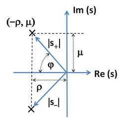
which shows for large enough values of βA0 the square root becomes the square root of a negative number, that is the square root becomes imaginary, and the pole positions are complex conjugate numbers, either s+ or s−; see Figure 2:

with

and

Using polar coordinates with the magnitude of the radius to the roots given by |s| (Figure 2):

and the angular coordinate φ is given by:

Tables of Laplace transforms show that the time response of such a system is composed of combinations of the two functions:


which is to say, the solutions are damped oscillations in time. In particular, the unit step response of the system is:[1]

which simplifies to

when A0 tends to infinity and the feedback factor β is one.
Notice that the damping of the response is set by ρ, that is, by the time constants of the open-loop amplifier. In contrast, the frequency of oscillation is set by μ, that is, by the feedback parameter through βA0. Because ρ is a sum of reciprocals of time constants, it is interesting to notice that ρ is dominated by the shorter of the two.
Results
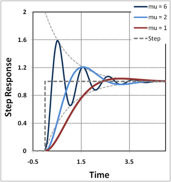
Figure 3 shows the time response to a unit step input for three values of the parameter μ. It can be seen that the frequency of oscillation increases with μ, but the oscillations are contained between the two asymptotes set by the exponentials [ 1 − exp (−ρt) ] and [ 1 + exp(−ρt) ]. These asymptotes are determined by ρ and therefore by the time constants of the open-loop amplifier, independent of feedback.
The phenomenon of oscillation about the final value is called ringing. The overshoot is the maximum swing above final value, and clearly increases with μ. Likewise, the undershoot is the minimum swing below final value, again increasing with μ. The settling time is the time for departures from final value to sink below some specified level, say 10% of final value.
The dependence of settling time upon μ is not obvious, and the approximation of a two-pole system probably is not accurate enough to make any real-world conclusions about feedback dependence of settling time. However, the asymptotes [ 1 − exp (−ρt) ] and [ 1 + exp (−ρt) ] clearly impact settling time, and they are controlled by the time constants of the open-loop amplifier, particularly the shorter of the two time constants. That suggests that a specification on settling time must be met by appropriate design of the open-loop amplifier.
The two major conclusions from this analysis are:
- Feedback controls the amplitude of oscillation about final value for a given open-loop amplifier and given values of open-loop time constants, τ1 and τ2.
- The open-loop amplifier decides settling time. It sets the time scale of Figure 3, and the faster the open-loop amplifier, the faster this time scale.
As an aside, it may be noted that real-world departures from this linear two-pole model occur due to two major complications: first, real amplifiers have more than two poles, as well as zeros; and second, real amplifiers are nonlinear, so their step response changes with signal amplitude.

Control of overshoot
How overshoot may be controlled by appropriate parameter choices is discussed next.
Using the equations above, the amount of overshoot can be found by differentiating the step response and finding its maximum value. The result for maximum step response Smax is:[2]

The final value of the step response is 1, so the exponential is the actual overshoot itself. It is clear the overshoot is zero if μ = 0, which is the condition:

This quadratic is solved for the ratio of time constants by setting x = ( τ1 / τ2 )1 / 2 with the result

Because β A0 >> 1, the 1 in the square root can be dropped, and the result is

In words, the first time constant must be much larger than the second. To be more adventurous than a design allowing for no overshoot we can introduce a factor α in the above relation:

and let α be set by the amount of overshoot that is acceptable.
Figure 4 illustrates the procedure. Comparing the top panel (α = 4) with the lower panel (α = 0.5) shows lower values for α increase the rate of response, but increase overshoot. The case α = 2 (center panel) is the maximally flat design that shows no peaking in the Bode gain vs. frequency plot. That design has the rule of thumb built-in safety margin to deal with non-ideal realities like multiple poles (or zeros), nonlinearity (signal amplitude dependence) and manufacturing variations, any of which can lead to too much overshoot. The adjustment of the pole separation (that is, setting α) is the subject of frequency compensation, and one such method is pole splitting.
Control of settling time
The amplitude of ringing in the step response in Figure 3 is governed by the damping factor exp ( −ρ t ). That is, if we specify some acceptable step response deviation from final value, say Δ, that is:

this condition is satisfied regardless of the value of β AOL provided the time is longer than the settling time, say tS, given by:[3]

where the τ1 >> τ2 is applicable because of the overshoot control condition, which makes τ1 = αβAOL τ2. Often the settling time condition is referred to by saying the settling period is inversely proportional to the unity gain bandwidth, because 1/(2π τ2) is close to this bandwidth for an amplifier with typical dominant pole compensation. However, this result is more precise than this rule of thumb. As an example of this formula, if Δ = 1/e4 = 1.8 %, the settling time condition is tS = 8 τ2.
In general, control of overshoot sets the time constant ratio, and settling time tS sets τ2.[4][5] [6]
Phase margin
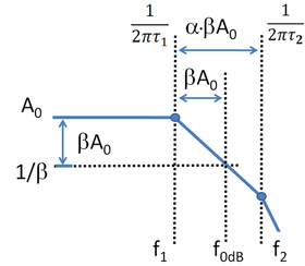
Next, the choice of pole ratio τ1/τ2 is related to the phase margin of the feedback amplifier.[7] The procedure outlined in the Bode plot article is followed. Figure 5 is the Bode gain plot for the two-pole amplifier in the range of frequencies up to the second pole position. The assumption behind Figure 5 is that the frequency f0 dB lies between the lowest pole at f1 = 1/(2πτ1) and the second pole at f2 = 1/(2πτ2). As indicated in Figure 5, this condition is satisfied for values of α ≥ 1.
Using Figure 5 the frequency (denoted by f0 dB) is found where the loop gain βA0 satisfies the unity gain or 0 dB condition, as defined by:

The slope of the downward leg of the gain plot is (20 dB/decade); for every factor of ten increase in frequency, the gain drops by the same factor:

The phase margin is the departure of the phase at f0 dB from −180°. Thus, the margin is:

Because f0 dB / f1 = βA0 >> 1, the term in f1 is 90°. That makes the phase margin:


In particular, for case α = 1, φm = 45°, and for α = 2, φm = 63.4°. Sansen[8] recommends α = 3, φm = 71.6° as a "good safety position to start with".
If α is increased by shortening τ2, the settling time tS also is shortened. If α is increased by lengthening τ1, the settling time tS is little altered. More commonly, both τ1 and τ2 change, for example if the technique of pole splitting is used.
As an aside, for an amplifier with more than two poles, the diagram of Figure 5 still may be made to fit the Bode plots by making f2 a fitting parameter, referred to as an "equivalent second pole" position.[9]
Formal mathematical description

This section provides a formal mathematical definition of step response in terms of the abstract mathematical concept of a dynamical system : all notations and assumptions required for the following description are listed here.

- is the evolution parameter of the system, called "time" for the sake of simplicity,
- is the state of the system at time , called "output" for the sake of simplicity,
- is the dynamical system evolution function,
- is the dynamical system initial state,
- is the Heaviside step function


Nonlinear dynamical system
For a general dynamical system, the step response is defined as follows:

It is the evolution function when the control inputs (or source term, or forcing inputs) are Heaviside functions: the notation emphasizes this concept showing H(t) as a subscript.
Linear dynamical system
For a linear time-invariant black box, let for notational convenience: the step response can be obtained by convolution of the Heaviside step function control and the impulse response h(t) of the system itself


which for an LTI system is equivalent to just integrating the latter. Conversely, for an LTI system, the derivative of the step response yields the impulse response:
- .

However, these simple relations are not true for a non-linear or time-variant system.[10]
See also
References and notes
- ↑ Benjamin C Kuo & Golnaraghi F (2003). Automatic control systems (Eighth ed.). New York: Wiley. p. 253. ISBN 0-471-13476-7.
- ↑ Benjamin C Kuo & Golnaraghi F. p. 259. ISBN 0-471-13476-7.
- ↑ This estimate is a bit conservative (long) because the factor 1 /sin(φ) in the overshoot contribution to S ( t ) has been replaced by 1 /sin(φ) ≈ 1.
- ↑ David A. Johns & Martin K W (1997). Analog integrated circuit design. New York: Wiley. pp. 234–235. ISBN 0-471-14448-7.
- ↑ Willy M C Sansen (2006). Analog design essentials. Dordrecht, The Netherlands: Springer. p. §0528 p. 163. ISBN 0-387-25746-2.
- ↑ According to Johns and Martin, op. cit., settling time is significant in switched-capacitor circuits, for example, where an op amp settling time must be less than half a clock period for sufficiently rapid charge transfer.
- ↑ The gain margin of the amplifier cannot be found using a two-pole model, because gain margin requires determination of the frequency f180 where the gain flips sign, and this never happens in a two-pole system. If we know f180 for the amplifier at hand, the gain margin can be found approximately, but f180 then depends on the third and higher pole positions, as does the gain margin, unlike the estimate of phase margin, which is a two-pole estimate.
- ↑ Willy M C Sansen. §0526 p. 162. ISBN 0-387-25746-2.
- ↑ Gaetano Palumbo & Pennisi S (2002). Feedback amplifiers: theory and design. Boston/Dordrecht/London: Kluwer Academic Press. pp. § 4.4 pp. 97–98. ISBN 0-7923-7643-9.
- ↑ Yuriy Shmaliy (2007). Continuous-Time Systems. Springer Science & Business Media. p. 46. ISBN 978-1-4020-6272-8.
Further reading
- Robert I. Demrow Settling time of operational amplifiers
- Cezmi Kayabasi Settling time measurement techniques achieving high precision at high speeds
- Vladimir Igorevic Arnol'd "Ordinary differential equations", various editions from MIT Press and from Springer Verlag, chapter 1 "Fundamental concepts"