Standard addition

How to make a standard addition plot

Example standard addition plot. This graph is an example of a standard addition plot used to determine the concentration of calcium in an unknown sample by atomic absorption spectroscopy. The point at zero concentration added Ca is the reading of the unknown, the other points are the readings after adding increasing amounts ('spikes') of standard solution. The absolute value of the x-intercept is the concentration of Ca in the unknown, in this case 1.69E-6 g/mL.

The method of standard addition is a type of quantitative analysis approach often used in analytical chemistry whereby the standard is added directly to the aliquots of analyzed sample. This method is used in situations where sample matrix also contributes to the analytical signal, a situation known as the matrix effect, thus making it impossible to compare the analytical signal between sample and standard using the traditional calibration curve approach.^[1]

Applications

Standard addition is frequently used in chemical instrumental analysis such as atomic absorption spectroscopy and gas chromatography.^[2]

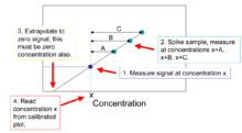
Suppose that the concentration of silver in samples of photographic waste is to be determined by atomic-absorption spectrometry. Using the calibration curve method, an analyst could calibrate the spectrometer with some aqueous solutions of a pure silver salt and use the resulting calibration graph in the determination of the silver in the test samples. This method is only valid, however, if a pure aqueous solution of silver, and a photographic waste sample containing the same concentration of silver, give the same absorbance values. In other words, in using pure solutions to establish the calibration graph it is assumed that there are no ‘matrix effects’, i.e. no reduction or enhancement of the silver absorbance signal by other components. In many areas of analysis such an assumption is frequently invalid. Matrix effects occur even with methods such as plasma spectrometry, which have a reputation for being relatively free from interferences. The method of standard additions is usually followed to eliminate matrix effects. Experimentally, equal volumes of the sample solution are taken, all but one are separately ‘spiked’ with known and different amounts of the analyte, and all are then diluted to the same volume. The instrument signals are then determined for all these solutions and the results plotted. As usual, the signal is plotted on the y-axis; in this case the x-axis is graduated in terms of the amounts of analyte added (either as an absolute weight or as a concentration). The (unweighted) regression line is calculated in the normal way, but space is provided for it to be extrapolated to the point on the x-axis at which y = 0. This negative intercept on the x-axis corresponds to the amount of the analyte in the test sample. This value is given by a/b, the ratio of the intercept and the slope of the regression line. Similarly in gas chromatography the following procedure is used: 1) The chromatogram of the unknown is recorded 2) a known amount of the analyte(s) of interest is added 3) the sample is analyzed again under the same conditions and the chromatogram is recorded. From the increase in the peak area (or peak height), the original concentration can be computed by extrapolation. The detector response must be a linear function of analyte concentration and yield no signal (other than background) at zero concentration of the analyte.

Procedure

A typical procedure involves preparing several solutions containing the same amount of unknown, but different amounts of standard. For example, five 25 mL volumetric flasks are each filled with 10 mL of the unknown. Then the standard is added in differing amounts, such as 0, 1, 2, 3, and 4 mL. The flasks are then diluted to the mark and mixed well.

The idea of this procedure is that the total concentration of the analyte is the combination of the unknown and the standard, and that the total concentration varies linearly. If the signal response is linear in this concentration range, then a plot similar to what is shown above is generated.

Error^[3]

The x-intercept gives the concentration of the unknown. Note this value is the diluted concentration. In the procedure section above, 10 mL of unknown was diluted to 25 mL. It is this diluted concentration that is found by the x-intercept. To find the original concentration of the unknown, one must back calculate that value. The error in the x-intercept is calculated as shown below.

$s_{x}={\frac {s_{y}}{|m|}}{\sqrt {{\frac {1}{n}}+{\frac {{\bar {y}}^{2}}{m^{2}\sum {(x_{i}-{\bar {x}})^{2}}}}}}$

$s_{y}$ is the standard deviation in the residuals $={\sqrt {{\frac {\sum {(y_{i}-mx_{i}-b)}^{2}}{n-2}}}}$
$m$ is the slope of the line
$b$ is the y-intercept of the line
$n$ is the number of standards
${\bar {y}}$ is the average measurement of the standards
$x_{i}$ are the concentrations of the standards
${\bar {x}}$ is the average concentration of the standards

References

↑ Harris, Daniel C. (2003). Quantitative Chemical Analysis 6th Edition. New York: W.H. Freeman.
↑ . doi:10.1021/ed057p703. Missing or empty |title= (help)
↑ Bruce, Graham R. (June 1999). "Estimates of Precision in a Standard Addition Analysis". Journal of Chemical Education. 76 (6): 805–807. doi:10.1021/ed076p805. Retrieved 8 March 2016.

Harris, Daniel C. (2003). Quantitative Chemical Analysis 6th Edition. New York: W.H. Freeman.

This article is issued from Wikipedia - version of the 11/26/2016. The text is available under the Creative Commons Attribution/Share Alike but additional terms may apply for the media files.

Standard addition

Applications

Procedure

Error[3]

See also

References

Error^[3]