Spin (physics)

This article is about spin in quantum mechanics. For rotation in classical mechanics, see angular momentum.

Standard Model of particle physics
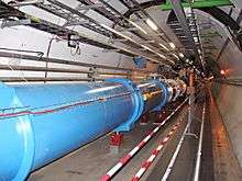Large Hadron Collider tunnel at CERN
Background Particle physics Standard Model Quantum field theory Gauge theory Spontaneous symmetry breaking Higgs mechanism
Constituents Electroweak interaction Quantum chromodynamics CKM matrix Standard Model mathematics
Limitations Strong CP problem Hierarchy problem Neutrino oscillations Physics beyond the Standard Model
Scientists Rutherford · Thomson · Chadwick · Bose · Sudarshan · Koshiba · Davis Jr. · Anderson · Fermi · Dirac · Feynman · Rubbia · Gell-Mann · Kendall · Taylor · Friedman · Powell · P. W. Anderson · Glashow · Meer · Cowan · Nambu · Chamberlain · Cabibbo · Schwartz · Perl · Majorana · Weinberg · Lee · Ward · Salam · Kobayashi · Maskawa · Yang · Yukawa · 't Hooft · Veltman · Gross · Politzer · Wilczek · Cronin · Fitch · Vleck · Higgs · Englert · Brout · Hagen · Guralnik · Kibble · Ting · Richter

In quantum mechanics and particle physics, spin is an intrinsic form of angular momentum carried by elementary particles, composite particles (hadrons), and atomic nuclei.^[1]^[2]

Spin is one of two types of angular momentum in quantum mechanics, the other being orbital angular momentum. The orbital angular momentum operator is the quantum-mechanical counterpart to the classical angular momentum of orbital revolution: it arises when a particle executes a rotating or twisting trajectory (such as when an electron orbits a nucleus).^[3]^[4] The existence of spin angular momentum is inferred from experiments, such as the Stern–Gerlach experiment, in which particles are observed to possess angular momentum that cannot be accounted for by orbital angular momentum alone.^[5]

In some ways, spin is like a vector quantity; it has a definite magnitude, and it has a "direction" (but quantization makes this "direction" different from the direction of an ordinary vector). All elementary particles of a given kind have the same magnitude of spin angular momentum, which is indicated by assigning the particle a spin quantum number.^[2]

The SI unit of spin is the (N·m·s) or (kg·m²·s⁻¹), just as with classical angular momentum. In practice, spin is given as a dimensionless spin quantum number by dividing the spin angular momentum by the reduced Planck constant $ħ$ , which has the same units of angular momentum. Very often, the "spin quantum number" is simply called "spin" leaving its meaning as the unitless "spin quantum number" to be inferred from context.

When combined with the spin-statistics theorem, the spin of electrons results in the Pauli exclusion principle, which in turn underlies the periodic table of chemical elements.

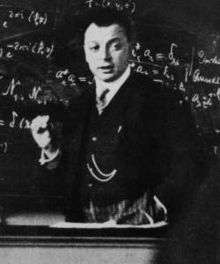
Wolfgang Pauli was the first to propose the concept of spin, but he did not name it. In 1925, Ralph Kronig, George Uhlenbeck and Samuel Goudsmit at Leiden University suggested an (erroneous) physical interpretation of particles spinning around their own axis. The mathematical theory was worked out in depth by Pauli in 1927. When Paul Dirac derived his relativistic quantum mechanics in 1928, electron spin was an essential part of it.

Quantum number

Main article: Spin quantum number

As the name suggests, spin was originally conceived as the rotation of a particle around some axis. This picture is correct so far as spin obeys the same mathematical laws as quantized angular momenta do. On the other hand, spin has some peculiar properties that distinguish it from orbital angular momenta:

Spin quantum numbers may take half-integer values.
Although the direction of its spin can be changed, an elementary particle cannot be made to spin faster or slower.
The spin of a charged particle is associated with a magnetic dipole moment with a $g$ -factor differing from 1. This could only occur classically if the internal charge of the particle were distributed differently from its mass.

The conventional definition of the spin quantum number, $s$ , is $s = n / 2$ , where $n$ can be any non-negative integer. Hence the allowed values of $s$ are 0, 1/2, 1, 3/2, 2, etc. The value of $s$ for an elementary particle depends only on the type of particle, and cannot be altered in any known way (in contrast to the spin direction described below). The spin angular momentum, $S$ , of any physical system is quantized. The allowed values of $S$ are

S=\hbar \,{\sqrt {s(s+1)}}={\frac {h}{4\pi }}\,{\sqrt {n(n+2)}},

where $h$ is the Planck constant and $\hbar$ is the reduced Planck constant. In contrast, orbital angular momentum can only take on integer values of $s$ ; i.e., even-numbered values of $n$ .

Fermions and bosons

Those particles with half-integer spins, such as 1/2, 3/2, 5/2, are known as fermions, while those particles with integer spins, such as 0, 1, 2, are known as bosons. The two families of particles obey different rules and broadly have different roles in the world around us. A key distinction between the two families is that fermions obey the Pauli exclusion principle; that is, there cannot be two identical fermions simultaneously having the same quantum numbers (meaning, roughly, having the same position, velocity and spin direction). In contrast, bosons obey the rules of Bose–Einstein statistics and have no such restriction, so they may "bunch together" even if in identical states. Also, composite particles can have spins different from their component particles. For example, a helium atom in the ground state has spin 0 and behaves like a boson, even though the quarks and electrons which make it up are all fermions.

This has profound practical applications:

Quarks and leptons (including electrons and neutrinos), which make up what is classically known as matter, are all fermions with spin 1/2. The common idea that "matter takes up space" actually comes from the Pauli exclusion principle acting on these particles to prevent the fermions that make up matter from being in the same quantum state. Further compaction would require electrons to occupy the same energy states, and therefore a kind of pressure (sometimes known as degeneracy pressure of electrons) acts to resist the fermions being overly close. It is also this pressure which prevents stars collapsing inwardly, and which, when it finally gives way under immense gravitational pressure in a dying massive star, triggers inward collapse into a black hole.

Elementary fermions with other spins (3/2, 5/2, etc.) are not known to exist, as of 2014.

Elementary particles which are thought of as carrying forces are all bosons with spin 1. They include the photon which carries the electromagnetic force, the gluon (strong force), and the W and Z bosons (weak force). The ability of bosons to occupy the same quantum state is used in the laser, which aligns many photons having the same quantum number (the same direction and frequency), superfluid liquid helium resulting from helium-4 atoms being bosons, and superconductivity where pairs of electrons (which individually are fermions) act as single composite bosons.

Elementary bosons with other spins (0, 2, 3 etc.) were not historically known to exist, although they have received considerable theoretical treatment and are well established within their respective mainstream theories. In particular, theoreticians have proposed the graviton (predicted to exist by some quantum gravity theories) with spin 2, and the Higgs boson (explaining electroweak symmetry breaking) with spin 0. Since 2013, the Higgs boson with spin 0 has been considered proven to exist.^[6] It is the first scalar particle (spin 0) known to exist in nature.

Theoretical and experimental studies have shown that the spin possessed by elementary particles cannot be explained by postulating that they are made up of even smaller particles rotating about a common center of mass analogous to a classical electron radius; as far as can be determined at present, these elementary particles have no inner structure. The spin of an elementary particle is therefore seen as a truly intrinsic physical property, akin to the particle's electric charge and rest mass.

Spin-statistics theorem

The proof that particles with half-integer spin (fermions) obey Fermi–Dirac statistics and the Pauli Exclusion Principle, and particles with integer spin (bosons) obey Bose–Einstein statistics, occupy "symmetric states", and thus can share quantum states, is known as the spin-statistics theorem. The theorem relies on both quantum mechanics and the theory of special relativity, and this connection between spin and statistics has been called "one of the most important applications of the special relativity theory".^[7]

Magnetic moments

Main article: Spin magnetic moment

Schematic diagram depicting the spin of the neutron as the black arrow and magnetic field lines associated with the neutron magnetic moment. The neutron has a negative magnetic moment. While the spin of the neutron is upward in this diagram, the magnetic field lines at the center of the dipole are downward.

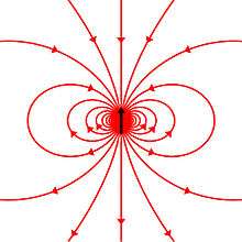
Particles with spin can possess a magnetic dipole moment, just like a rotating electrically charged body in classical electrodynamics. These magnetic moments can be experimentally observed in several ways, e.g. by the deflection of particles by inhomogeneous magnetic fields in a Stern–Gerlach experiment, or by measuring the magnetic fields generated by the particles themselves.

The intrinsic magnetic moment $μ$ of a spin 1/2 particle with charge $q$ , mass $m$ , and spin angular momentum $S$ , is^[8]

\boldsymbol{\mu} = \frac{g_s q}{2m} \mathbf{S}

where the dimensionless quantity $g s$ is called the spin $g$ -factor. For exclusively orbital rotations it would be 1 (assuming that the mass and the charge occupy spheres of equal radius).

The electron, being a charged elementary particle, possesses a nonzero magnetic moment. One of the triumphs of the theory of quantum electrodynamics is its accurate prediction of the electron $g$ -factor, which has been experimentally determined to have the value 2999799768069563780♠−2.0023193043622(15), with the digits in parentheses denoting measurement uncertainty in the last two digits at one standard deviation.^[9] The value of 2 arises from the Dirac equation, a fundamental equation connecting the electron's spin with its electromagnetic properties, and the correction of 6997231930400000000♠0.002319304... arises from the electron's interaction with the surrounding electromagnetic field, including its own field.^[10] Composite particles also possess magnetic moments associated with their spin. In particular, the neutron possesses a non-zero magnetic moment despite being electrically neutral. This fact was an early indication that the neutron is not an elementary particle. In fact, it is made up of quarks, which are electrically charged particles. The magnetic moment of the neutron comes from the spins of the individual quarks and their orbital motions.

Neutrinos are both elementary and electrically neutral. The minimally extended Standard Model that takes into account non-zero neutrino masses predicts neutrino magnetic moments of:^[11]^[12]^[13]

\mu_{\nu}\approx 3\times 10^{-19}\mu_\mathrm{B}\frac{m_{\nu}}{\text{eV}}

where the $μ ν$ are the neutrino magnetic moments, $m ν$ are the neutrino masses, and $μ B$ is the Bohr magneton. New physics above the electroweak scale could, however, lead to significantly higher neutrino magnetic moments. It can be shown in a model independent way that neutrino magnetic moments larger than about 10⁻¹⁴ $μ B$ are unnatural, because they would also lead to large radiative contributions to the neutrino mass. Since the neutrino masses cannot exceed about 1 eV, these radiative corrections must then be assumed to be fine tuned to cancel out to a large degree.^[14]

The measurement of neutrino magnetic moments is an active area of research. As of 2001, the latest experimental results have put the neutrino magnetic moment at less than 6990120000000000000♠1.2×10⁻¹⁰ times the electron's magnetic moment.

In ordinary materials, the magnetic dipole moments of individual atoms produce magnetic fields that cancel one another, because each dipole points in a random direction. Ferromagnetic materials below their Curie temperature, however, exhibit magnetic domains in which the atomic dipole moments are locally aligned, producing a macroscopic, non-zero magnetic field from the domain. These are the ordinary "magnets" with which we are all familiar.

In paramagnetic materials, the magnetic dipole moments of individual atoms spontaneously align with an externally applied magnetic field. In diamagnetic materials, on the other hand, the magnetic dipole moments of individual atoms spontaneously align oppositely to any externally applied magnetic field, even if it requires energy to do so.

The study of the behavior of such "spin models" is a thriving area of research in condensed matter physics. For instance, the Ising model describes spins (dipoles) that have only two possible states, up and down, whereas in the Heisenberg model the spin vector is allowed to point in any direction. These models have many interesting properties, which have led to interesting results in the theory of phase transitions.

Direction

Further information: Angular momentum operator

Spin projection quantum number and multiplicity

In classical mechanics, the angular momentum of a particle possesses not only a magnitude (how fast the body is rotating), but also a direction (either up or down on the axis of rotation of the particle). Quantum mechanical spin also contains information about direction, but in a more subtle form. Quantum mechanics states that the component of angular momentum measured along any direction can only take on the values ^[15]

S_i = \hbar s_i, \quad s_i \in \{ - s, -(s-1), \dots, s-1, s \} \,\!

where $S i$ is the spin component along the $i$ -axis (either $x$ , $y$ , or $z$ ), $s i$ is the spin projection quantum number along the $i$ -axis, and $s$ is the principal spin quantum number (discussed in the previous section). Conventionally the direction chosen is the $z$ -axis:

S_z = \hbar s_z, \quad s_z \in \{ - s, -(s-1), \dots, s - 1, s \} \,\!

where $S z$ is the spin component along the $z$ -axis, $s z$ is the spin projection quantum number along the $z$ -axis.

One can see that there are $2 s + 1$ possible values of $s z$ . The number " $2 s + 1$ " is the multiplicity of the spin system. For example, there are only two possible values for a spin-1/2 particle: $s z = + 1 / 2$ and $s z = - 1 / 2$ . These correspond to quantum states in which the spin is pointing in the +z or −z directions respectively, and are often referred to as "spin up" and "spin down". For a spin-3/2 particle, like a delta baryon, the possible values are +3/2, +1/2, −1/2, −3/2.

Vector

A single point in space can spin continuously without becoming tangled. Notice that after a 360-degree rotation, the spiral flips between clockwise and counterclockwise orientations. It returns to its original configuration after spinning a full 720 degrees.

For a given quantum state, one could think of a spin vector ${\textstyle \langle S\rangle }$ whose components are the expectation values of the spin components along each axis, i.e., ${\textstyle \langle S\rangle =[\langle S_{x}\rangle ,\langle S_{y}\rangle ,\langle S_{z}\rangle ]}$ . This vector then would describe the "direction" in which the spin is pointing, corresponding to the classical concept of the axis of rotation. It turns out that the spin vector is not very useful in actual quantum mechanical calculations, because it cannot be measured directly: $s x$ , $s y$ and $s z$ cannot possess simultaneous definite values, because of a quantum uncertainty relation between them. However, for statistically large collections of particles that have been placed in the same pure quantum state, such as through the use of a Stern–Gerlach apparatus, the spin vector does have a well-defined experimental meaning: It specifies the direction in ordinary space in which a subsequent detector must be oriented in order to achieve the maximum possible probability (100%) of detecting every particle in the collection. For spin-1/2 particles, this maximum probability drops off smoothly as the angle between the spin vector and the detector increases, until at an angle of 180 degrees—that is, for detectors oriented in the opposite direction to the spin vector—the expectation of detecting particles from the collection reaches a minimum of 0%.

As a qualitative concept, the spin vector is often handy because it is easy to picture classically. For instance, quantum mechanical spin can exhibit phenomena analogous to classical gyroscopic effects. For example, one can exert a kind of "torque" on an electron by putting it in a magnetic field (the field acts upon the electron's intrinsic magnetic dipole moment—see the following section). The result is that the spin vector undergoes precession, just like a classical gyroscope. This phenomenon is known as electron spin resonance (ESR). The equivalent behaviour of protons in atomic nuclei is used in nuclear magnetic resonance (NMR) spectroscopy and imaging.

Mathematically, quantum mechanical spin states are described by vector-like objects known as spinors. There are subtle differences between the behavior of spinors and vectors under coordinate rotations. For example, rotating a spin-1/2 particle by 360 degrees does not bring it back to the same quantum state, but to the state with the opposite quantum phase; this is detectable, in principle, with interference experiments. To return the particle to its exact original state, one needs a 720-degree rotation. (The Plate trick and Mobius strip give non-quantum analogies.) A spin-zero particle can only have a single quantum state, even after torque is applied. Rotating a spin-2 particle 180 degrees can bring it back to the same quantum state and a spin-4 particle should be rotated 90 degrees to bring it back to the same quantum state. The spin 2 particle can be analogous to a straight stick that looks the same even after it is rotated 180 degrees and a spin 0 particle can be imagined as sphere which looks the same after whatever angle it is turned through.

Mathematical formulation

Operator

Spin obeys commutation relations analogous to those of the orbital angular momentum:

[S_{i},S_{j}]=i\hbar \varepsilon _{ijk}S_{k}

where $ε ijk$ is the Levi-Civita symbol, and the expression is summed over the $k$ th index. It follows (as with angular momentum) that the eigenvectors of $S 2$ and $S z$ (expressed as kets in the total $S$ basis) are:

{\begin{aligned}S^{2}|s,m_{s}\rangle &=\hbar ^{2}s(s+1)|s,m_{s}\rangle \\S_{z}|s,m_{s}\rangle &=\hbar m_{s}|s,m_{s}\rangle .\end{aligned}}

The spin raising and lowering operators acting on these eigenvectors give:

S_{\pm }|s,m_{s}\rangle =\hbar {\sqrt {s(s+1)-m_{s}(m_{s}\pm 1)}}|s,m_{s}\pm 1\rangle

where $S \pm = S x \pm i S y$ .

But unlike orbital angular momentum the eigenvectors are not spherical harmonics. They are not functions of $θ$ and $φ$ . There is also no reason to exclude half-integer values of $s$ and $m s$ .

In addition to their other properties, all quantum mechanical particles possess an intrinsic spin (though it may have the intrinsic spin 0, too). The spin is quantized in units of the reduced Planck constant, such that the state function of the particle is, say, not $ψ = ψ (r)$ , but $ψ = ψ (r, σ)$ where $σ$ is out of the following discrete set of values:

\sigma \in \{-s\hbar, -(s - 1)\hbar, \cdots, +(s - 1)\hbar, +s\hbar\}.

One distinguishes bosons (integer spin) and fermions (half-integer spin). The total angular momentum conserved in interaction processes is then the sum of the orbital angular momentum and the spin.

Pauli matrices

Main article: Pauli matrices

The quantum mechanical operators associated with spin-1/2 observables are:

{\hat {{\mathbf {S}}}}={\frac {\hbar }{2}}{\boldsymbol {\sigma }}

where in Cartesian components:

S_{x}={\hbar \over 2}\sigma _{x},\quad S_{y}={\hbar \over 2}\sigma _{y},\quad S_{z}={\hbar \over 2}\sigma _{z}\,.

For the special case of spin-1/2 particles, $σ x$ , $σ y$ and $σ z$ are the three Pauli matrices, given by:

\sigma _{x}={\begin{pmatrix}0&1\\1&0\end{pmatrix}}\,\quad \sigma _{y}={\begin{pmatrix}0&-i\\i&0\end{pmatrix}}\,\quad \sigma _{z}={\begin{pmatrix}1&0\\0&-1\end{pmatrix}}\,.

Pauli exclusion principle

For systems of $N$ identical particles this is related to the Pauli exclusion principle, which states that by interchanges of any two of the $N$ particles one must have

\psi ( \cdots \mathbf r_i,\sigma_i\cdots \mathbf r_j,\sigma_j\cdots ) = (-1)^{2s}\psi ( \cdots \mathbf r_j,\sigma_j\cdots \mathbf r_i,\sigma_i\cdots ) .

Thus, for bosons the prefactor $(-1) 2 s$ will reduce to +1, for fermions to −1. In quantum mechanics all particles are either bosons or fermions. In some speculative relativistic quantum field theories "supersymmetric" particles also exist, where linear combinations of bosonic and fermionic components appear. In two dimensions, the prefactor $(-1) 2 s$ can be replaced by any complex number of magnitude 1 such as in the anyon.

The above permutation postulate for $N$ -particle state functions has most-important consequences in daily life, e.g. the periodic table of the chemical elements.

Rotations

As described above, quantum mechanics states that components of angular momentum measured along any direction can only take a number of discrete values. The most convenient quantum mechanical description of particle's spin is therefore with a set of complex numbers corresponding to amplitudes of finding a given value of projection of its intrinsic angular momentum on a given axis. For instance, for a spin-1/2 particle, we would need two numbers $a \pm 1 / 2$ , giving amplitudes of finding it with projection of angular momentum equal to $ħ / 2$ and $- ħ / 2$ , satisfying the requirement

\left|a_\frac{1}{2}\right|^2 + \left|a_{-\frac{1}{2}}\right|^2 \, = 1.

For a generic particle with spin $s$ , we would need $2 s + 1$ such parameters. Since these numbers depend on the choice of the axis, they transform into each other non-trivially when this axis is rotated. It's clear that the transformation law must be linear, so we can represent it by associating a matrix with each rotation, and the product of two transformation matrices corresponding to rotations A and B must be equal (up to phase) to the matrix representing rotation AB. Further, rotations preserve the quantum mechanical inner product, and so should our transformation matrices:

\sum_{m=-j}^{j} a_m^* b_m = \sum_{m=-j}^{j} \left(\sum_{n=-j}^j U_{nm} a_n\right)^* \left(\sum_{k=-j}^j U_{km} b_k\right)

\sum_{n=-j}^j \sum_{k=-j}^j U_{np}^* U_{kq} = \delta_{pq}.

Mathematically speaking, these matrices furnish a unitary projective representation of the rotation group SO(3). Each such representation corresponds to a representation of the covering group of SO(3), which is SU(2).^[16] There is one $n$ -dimensional irreducible representation of SU(2) for each dimension, though this representation is $n$ -dimensional real for odd $n$ and $n$ -dimensional complex for even $n$ (hence of real dimension $2 n$ ). For a rotation by angle $θ$ in the plane with normal vector ${\textstyle {\hat {\boldsymbol {\theta }}}}$ , $U$ can be written

U=e^{{-{\frac {i}{\hbar }}{\boldsymbol {\theta }}\cdot {\mathbf {S}}}},

where ${\textstyle {\boldsymbol {\theta }}=\theta {\hat {\boldsymbol {\theta }}}}$ , and $S$ is the vector of spin operators.

(Click "show" at right to see a proof or "hide" to hide it.)

Working in the coordinate system where ${\textstyle {\hat {\theta }}={\hat {z}}}$ , we would like to show that $S x$ and $S y$ are rotated into each other by the angle $θ$ . Starting with $S x$ . Using units where $ħ = 1$ :

$\begin{align} S_x \rightarrow U^\dagger S_x U &{}= e^{i \theta S_z} S_x e^{-i \theta S_z} \\ &{} = S_x + (i \theta) [S_z, S_x] + \left(\frac{1}{2!}\right) (i \theta)^2 [S_z, [S_z, S_x]] + \left(\frac{1}{3!}\right) (i \theta)^3 [S_z, [S_z, [S_z, S_x]]] + \cdots\\ \end{align}$

Using the spin operator commutation relations, we see that the commutators evaluate to $i S y$ for the odd terms in the series, and to $S x$ for all of the even terms. Thus:

$\begin{align} U^\dagger S_x U &{}= S_x \left[ 1 - \frac{\theta^2}{2!} + ... \right] - S_y \left[ \theta - \frac{\theta^3}{3!} \cdots \right] \\ &{} = S_x \cos\theta - S_y \sin\theta\\ \end{align}$

as expected. Note that since we only relied on the spin operator commutation relations, this proof holds for any dimension (i.e., for any principal spin quantum number $s$ ).^[17]

A generic rotation in 3-dimensional space can be built by compounding operators of this type using Euler angles:

{\mathcal {R}}(\alpha ,\beta ,\gamma )=e^{-i\alpha S_{z}}e^{-i\beta S_{y}}e^{-i\gamma S_{z}}

An irreducible representation of this group of operators is furnished by the Wigner D-matrix:

D^s_{m'm}(\alpha,\beta,\gamma) \equiv \langle sm' | \mathcal{R}(\alpha,\beta,\gamma)| sm \rangle = e^{-im'\alpha} d^s_{m'm}(\beta)e^{-i m\gamma},

where

d^s_{m'm}(\beta)= \langle sm' |e^{-i\beta s_y} | sm \rangle

is Wigner's small d-matrix. Note that for $γ = 2π$ and $α = β = 0$ ; i.e., a full rotation about the $z$ -axis, the Wigner D-matrix elements become

D^s_{m'm}(0,0,2\pi) = d^s_{m'm}(0) e^{-i m 2 \pi} = \delta_{m'm} (-1)^{2m}.

Recalling that a generic spin state can be written as a superposition of states with definite $m$ , we see that if $s$ is an integer, the values of $m$ are all integers, and this matrix corresponds to the identity operator. However, if $s$ is a half-integer, the values of $m$ are also all half-integers, giving $(-1) 2 m = -1$ for all $m$ , and hence upon rotation by 2 $π$ the state picks up a minus sign. This fact is a crucial element of the proof of the spin-statistics theorem.

Lorentz transformations

We could try the same approach to determine the behavior of spin under general Lorentz transformations, but we would immediately discover a major obstacle. Unlike SO(3), the group of Lorentz transformations SO(3,1) is non-compact and therefore does not have any faithful, unitary, finite-dimensional representations.

In case of spin-1/2 particles, it is possible to find a construction that includes both a finite-dimensional representation and a scalar product that is preserved by this representation. We associate a 4-component Dirac spinor $ψ$ with each particle. These spinors transform under Lorentz transformations according to the law

\psi '=\exp {\left({\tfrac {1}{8}}\omega _{\mu \nu }[\gamma _{\mu },\gamma _{\nu }]\right)}\psi

where $γ ν$ are gamma matrices and $ω μν$ is an antisymmetric 4 × 4 matrix parametrizing the transformation. It can be shown that the scalar product

\langle\psi|\phi\rangle = \bar{\psi}\phi = \psi^{\dagger}\gamma_0\phi

is preserved. It is not, however, positive definite, so the representation is not unitary.

Measurement of spin along the $x$ -, $y$ -, or $z$ -axes

Each of the (Hermitian) Pauli matrices has two eigenvalues, +1 and −1. The corresponding normalized eigenvectors are:

\begin{array}{lclc} \psi_{x+}=\displaystyle\frac{1}{\sqrt{2}}\!\!\!\!\! & \begin{pmatrix}{1}\\{1}\end{pmatrix}, & \psi_{x-}=\displaystyle\frac{1}{\sqrt{2}}\!\!\!\!\! & \begin{pmatrix}{1}\\{-1}\end{pmatrix}, \\ \psi_{y+}=\displaystyle\frac{1}{\sqrt{2}}\!\!\!\!\! & \begin{pmatrix}{1}\\{i}\end{pmatrix}, & \psi_{y-}=\displaystyle\frac{1}{\sqrt{2}}\!\!\!\!\! & \begin{pmatrix}{1}\\{-i}\end{pmatrix}, \\ \psi_{z+}= & \begin{pmatrix}{1}\\{0}\end{pmatrix}, & \psi_{z-}= & \begin{pmatrix}{0}\\{1}\end{pmatrix}. \end{array}

By the postulates of quantum mechanics, an experiment designed to measure the electron spin on the $x$ -, $y$ -, or $z$ -axis can only yield an eigenvalue of the corresponding spin operator ( $S x$ , $S y$ or $S z$ ) on that axis, i.e. $ħ / 2$ or $- ħ / 2$ . The quantum state of a particle (with respect to spin), can be represented by a two component spinor:

\psi = \begin{pmatrix} {a+bi}\\{c+di}\end{pmatrix}.

When the spin of this particle is measured with respect to a given axis (in this example, the $x$ -axis), the probability that its spin will be measured as $ħ / 2$ is just ${\textstyle \left\vert \langle \psi _{x+}\vert \psi \rangle \right\vert ^{2}}$ . Correspondingly, the probability that its spin will be measured as $- ħ / 2$ is just ${\textstyle \left\vert \langle \psi _{x-}\vert \psi \rangle \right\vert ^{2}}$ . Following the measurement, the spin state of the particle will collapse into the corresponding eigenstate. As a result, if the particle's spin along a given axis has been measured to have a given eigenvalue, all measurements will yield the same eigenvalue (since ${\textstyle \left\vert \langle \psi _{x+}\vert \psi _{x+}\rangle \right\vert ^{2}=1}$ , etc), provided that no measurements of the spin are made along other axes.

Measurement of spin along an arbitrary axis

The operator to measure spin along an arbitrary axis direction is easily obtained from the Pauli spin matrices. Let $u = (u x, u y, u z)$ be an arbitrary unit vector. Then the operator for spin in this direction is simply

S_u = \frac{\hbar}{2}(u_x\sigma_x + u_y\sigma_y + u_z\sigma_z)

The operator $S u$ has eigenvalues of $\pm ħ / 2$ , just like the usual spin matrices. This method of finding the operator for spin in an arbitrary direction generalizes to higher spin states, one takes the dot product of the direction with a vector of the three operators for the three $x$ -, $y$ -, $z$ -axis directions.

A normalized spinor for spin-1/2 in the $(u x, u y, u z)$ direction (which works for all spin states except spin down where it will give 0/0), is:

\frac{1}{\sqrt{2+2u_z}}\begin{pmatrix} 1+u_z \\ u_x+iu_y \end{pmatrix}.

The above spinor is obtained in the usual way by diagonalizing the $σ u$ matrix and finding the eigenstates corresponding to the eigenvalues. In quantum mechanics, vectors are termed "normalized" when multiplied by a normalizing factor, which results in the vector having a length of unity.

Compatibility of spin measurements

Since the Pauli matrices do not commute, measurements of spin along the different axes are incompatible. This means that if, for example, we know the spin along the $x$ -axis, and we then measure the spin along the $y$ -axis, we have invalidated our previous knowledge of the $x$ -axis spin. This can be seen from the property of the eigenvectors (i.e. eigenstates) of the Pauli matrices that:

\left\vert \langle \psi _{x\pm }\mid \psi _{y\pm }\rangle \right\vert ^{2}=\left\vert \langle \psi _{x\pm }\mid \psi _{z\pm }\rangle \right\vert ^{2}=\left\vert \langle \psi _{y\pm }\mid \psi _{z\pm }\rangle \right\vert ^{2}={\tfrac {1}{2}}.

So when physicists measure the spin of a particle along the $x$ -axis as, for example, $ħ / 2$ , the particle's spin state collapses into the eigenstate ${\textstyle \mid \psi _{x+}\rangle }$ . When we then subsequently measure the particle's spin along the $y$ -axis, the spin state will now collapse into either ${\textstyle \mid \psi _{y+}\rangle }$ or ${\textstyle \mid \psi _{y-}\rangle }$ , each with probability 1/2. Let us say, in our example, that we measure $- ħ / 2$ . When we now return to measure the particle's spin along the $x$ -axis again, the probabilities that we will measure $ħ / 2$ or $- ħ / 2$ are each 1/2 (i.e. they are ${\textstyle \left\vert \langle \psi _{x+}\mid \psi _{y-}\rangle \right\vert ^{2}}$ and ${\textstyle \left\vert \langle \psi _{x-}\mid \psi _{y-}\rangle \right\vert ^{2}}$ respectively). This implies that the original measurement of the spin along the x-axis is no longer valid, since the spin along the $x$ -axis will now be measured to have either eigenvalue with equal probability.

Higher spins

The spin-1/2 operator $S = ħ / 2 σ$ form the fundamental representation of SU(2). By taking Kronecker products of this representation with itself repeatedly, one may construct all higher irreducible representations. That is, the resulting spin operators for higher spin systems in three spatial dimensions, for arbitrarily large $s$ , can be calculated using this spin operator and ladder operators.

The resulting spin matrices for spin 1 are:

{\begin{aligned}S_{x}&={\frac {\hbar }{{\sqrt {2}}}}{\begin{pmatrix}0&1&0\\1&0&1\\0&1&0\end{pmatrix}}\,\\S_{y}&={\frac {\hbar }{{\sqrt {2}}}}{\begin{pmatrix}0&-i&0\\i&0&-i\\0&i&0\end{pmatrix}}\,\\S_{z}&=\hbar {\begin{pmatrix}1&0&0\\0&0&0\\0&0&-1\end{pmatrix}}\,\end{aligned}}

for spin 3/2 they are

{\begin{aligned}S_{x}&={\frac \hbar 2}{\begin{pmatrix}0&{\sqrt {3}}&0&0\\{\sqrt {3}}&0&2&0\\0&2&0&{\sqrt {3}}\\0&0&{\sqrt {3}}&0\end{pmatrix}}\,\\S_{y}&={\frac \hbar 2}{\begin{pmatrix}0&-i{\sqrt {3}}&0&0\\i{\sqrt {3}}&0&-2i&0\\0&2i&0&-i{\sqrt {3}}\\0&0&i{\sqrt {3}}&0\end{pmatrix}}\,\\S_{z}&={\frac \hbar 2}{\begin{pmatrix}3&0&0&0\\0&1&0&0\\0&0&-1&0\\0&0&0&-3\end{pmatrix}}\,\end{aligned}}

and for spin 5/2 they are

{\begin{aligned}S_{x}&={\frac \hbar 2}{\begin{pmatrix}0&{\sqrt {5}}&0&0&0&0\\{\sqrt {5}}&0&2{\sqrt {2}}&0&0&0\\0&2{\sqrt {2}}&0&3&0&0\\0&0&3&0&2{\sqrt {2}}&0\\0&0&0&2{\sqrt {2}}&0&{\sqrt {5}}\\0&0&0&0&{\sqrt {5}}&0\end{pmatrix}}\,\\S_{y}&={\frac \hbar 2}{\begin{pmatrix}0&-i{\sqrt {5}}&0&0&0&0\\i{\sqrt {5}}&0&-2i{\sqrt {2}}&0&0&0\\0&2i{\sqrt {2}}&0&-3i&0&0\\0&0&3i&0&-2i{\sqrt {2}}&0\\0&0&0&2i{\sqrt {2}}&0&-i{\sqrt {5}}\\0&0&0&0&i{\sqrt {5}}&0\end{pmatrix}}\,\\S_{z}&={\frac \hbar 2}{\begin{pmatrix}5&0&0&0&0&0\\0&3&0&0&0&0\\0&0&1&0&0&0\\0&0&0&-1&0&0\\0&0&0&0&-3&0\\0&0&0&0&0&-5\end{pmatrix}}\,.\end{aligned}}

The generalization of these matrices for arbitrary $s$ is

{\begin{aligned}\left(S_{x}\right)_{{ab}}&={\frac {\hbar }{2}}(\delta _{{a,b+1}}+\delta _{{a+1,b}}){\sqrt {(s+1)(a+b-1)-ab}}\,\\\left(S_{y}\right)_{{ab}}&={\frac {\hbar }{2i}}(\delta _{{a,b+1}}-\delta _{{a+1,b}}){\sqrt {(s+1)(a+b-1)-ab}}\,\quad 1\leq a,b\leq 2s+1\,\\\left(S_{z}\right)_{{ab}}&=\hbar (s+1-a)\delta _{{a,b}}=\hbar (s+1-b)\delta _{{a,b}}\,.\end{aligned}}

Also useful in the quantum mechanics of multiparticle systems, the general Pauli group $G n$ is defined to consist of all $n$ -fold tensor products of Pauli matrices.

The analog formula of Euler's formula in terms of the Pauli matrices:

e^{{i\theta ({\hat {{\mathbf {n}}}}\cdot {\boldsymbol {\sigma }})}}=I\cos \theta +i({\hat {{\mathbf {n}}}}\cdot {\boldsymbol {\sigma }})\sin \theta \,

for higher spins is tractable, but less simple.^[18]

Parity

In tables of the spin quantum number $s$ for nuclei or particles, the spin is often followed by a "+" or "−". This refers to the parity with "+" for even parity (wave function unchanged by spatial inversion) and "−" for odd parity (wave function negated by spatial inversion). For example, see the isotopes of bismuth.

Applications

Spin has important theoretical implications and practical applications. Well-established direct applications of spin include:

Nuclear magnetic resonance (NMR) spectroscopy in chemistry;
Electron spin resonance spectroscopy in chemistry and physics;
Magnetic resonance imaging (MRI) in medicine, a type of applied NMR, which relies on proton spin density;
Giant magnetoresistive (GMR) drive head technology in modern hard disks.

Electron spin plays an important role in magnetism, with applications for instance in computer memories. The manipulation of nuclear spin by radiofrequency waves (nuclear magnetic resonance) is important in chemical spectroscopy and medical imaging.

Spin-orbit coupling leads to the fine structure of atomic spectra, which is used in atomic clocks and in the modern definition of the second. Precise measurements of the $g$ -factor of the electron have played an important role in the development and verification of quantum electrodynamics. Photon spin is associated with the polarization of light.

An emerging application of spin is as a binary information carrier in spin transistors. The original concept, proposed in 1990, is known as Datta-Das spin transistor.^[19] Electronics based on spin transistors are referred to as spintronics. The manipulation of spin in dilute magnetic semiconductor materials, such as metal-doped ZnO or TiO₂ imparts a further degree of freedom and has the potential to facilitate the fabrication of more efficient electronics.^[20]

There are many indirect applications and manifestations of spin and the associated Pauli exclusion principle, starting with the periodic table of chemistry.

History

Spin was first discovered in the context of the emission spectrum of alkali metals. In 1924 Wolfgang Pauli introduced what he called a "two-valued quantum degree of freedom" associated with the electron in the outermost shell. This allowed him to formulate the Pauli exclusion principle, stating that no two electrons can share the same quantum state at the same time.

Wolfgang Pauli lecturing

The physical interpretation of Pauli's "degree of freedom" was initially unknown. Ralph Kronig, one of Landé's assistants, suggested in early 1925 that it was produced by the self-rotation of the electron. When Pauli heard about the idea, he criticized it severely, noting that the electron's hypothetical surface would have to be moving faster than the speed of light in order for it to rotate quickly enough to produce the necessary angular momentum. This would violate the theory of relativity. Largely due to Pauli's criticism, Kronig decided not to publish his idea.

In the autumn of 1925, the same thought came to two Dutch physicists, George Uhlenbeck and Samuel Goudsmit at Leiden University. Under the advice of Paul Ehrenfest, they published their results. It met a favorable response, especially after Llewellyn Thomas managed to resolve a factor-of-two discrepancy between experimental results and Uhlenbeck and Goudsmit's calculations (and Kronig's unpublished results). This discrepancy was due to the orientation of the electron's tangent frame, in addition to its position.

Mathematically speaking, a fiber bundle description is needed. The tangent bundle effect is additive and relativistic; that is, it vanishes if $c$ goes to infinity. It is one half of the value obtained without regard for the tangent space orientation, but with opposite sign. Thus the combined effect differs from the latter by a factor two (Thomas precession).

Despite his initial objections, Pauli formalized the theory of spin in 1927, using the modern theory of quantum mechanics invented by Schrödinger and Heisenberg. He pioneered the use of Pauli matrices as a representation of the spin operators, and introduced a two-component spinor wave-function.

Pauli's theory of spin was non-relativistic. However, in 1928, Paul Dirac published the Dirac equation, which described the relativistic electron. In the Dirac equation, a four-component spinor (known as a "Dirac spinor") was used for the electron wave-function. In 1940, Pauli proved the spin-statistics theorem, which states that fermions have half-integer spin and bosons have integer spin.

In retrospect, the first direct experimental evidence of the electron spin was the Stern–Gerlach experiment of 1922. However, the correct explanation of this experiment was only given in 1927.^[21]

References

↑ Merzbacher, Eugen (1998). Quantum Mechanics (3rd ed.). pp. 372–3.
1 2 Griffiths, David (2005). Introduction to Quantum Mechanics (2nd ed.). pp. 183–4.
↑ "Angular Momentum Operator Algebra", class notes by Michael Fowler
↑ A modern approach to quantum mechanics, by Townsend, p. 31 and p. 80
↑ Eisberg, Robert; Resnick, Robert (1985). Quantum Physics of Atoms, Molecules, Solids, Nuclei, and Particles (2nd ed.). pp. 272–3.
↑ Information about Higgs Boson in CERN's official website.
↑ Pauli, Wolfgang (1940). "The Connection Between Spin and Statistics" (PDF). Phys. Rev. 58 (8): 716–722. Bibcode:1940PhRv...58..716P. doi:10.1103/PhysRev.58.716.
↑ Physics of Atoms and Molecules, B.H. Bransden, C.J.Joachain, Longman, 1983, ISBN 0-582-44401-2
↑ "CODATA Value: electron g factor". The NIST Reference on Constants, Units, and Uncertainty. NIST. 2006. Retrieved 2013-11-15.
↑ R.P. Feynman (1985). "Electrons and Their Interactions". QED: The Strange Theory of Light and Matter. Princeton, New Jersey: Princeton University Press. p. 115. ISBN 0-691-08388-6.

"After some years, it was discovered that this value [ $- g / 2$ ] was not exactly 1, but slightly more—something like 1.00116. This correction was worked out for the first time in 1948 by Schwinger as $j * j$ divided by 2 pi [sic] [where $j$ is the square root of the fine-structure constant], and was due to an alternative way the electron can go from place to place: instead of going directly from one point to another, the electron goes along for a while and suddenly emits a photon; then (horrors!) it absorbs its own photon."
↑ W.J. Marciano, A.I. Sanda (1977). "Exotic decays of the muon and heavy leptons in gauge theories". Physics Letters. B67 (3): 303–305. Bibcode:1977PhLB...67..303M. doi:10.1016/0370-2693(77)90377-X.
↑ B.W. Lee, R.E. Shrock (1977). "Natural suppression of symmetry violation in gauge theories: Muon- and electron-lepton-number nonconservation". Physical Review. D16 (5): 1444–1473. Bibcode:1977PhRvD..16.1444L. doi:10.1103/PhysRevD.16.1444.
↑ K. Fujikawa, R. E. Shrock (1980). "Magnetic Moment of a Massive Neutrino and Neutrino-Spin Rotation". Physical Review Letters. 45 (12): 963–966. Bibcode:1980PhRvL..45..963F. doi:10.1103/PhysRevLett.45.963.
↑ N.F. Bell; Cirigliano, V.; Ramsey-Musolf, M.; Vogel, P.; Wise, Mark; et al. (2005). "How Magnetic is the Dirac Neutrino?". Physical Review Letters. 95 (15): 151802. arXiv:hep-ph/0504134. Bibcode:2005PhRvL..95o1802B. doi:10.1103/PhysRevLett.95.151802. PMID 16241715.
↑ Quanta: A handbook of concepts, P.W. Atkins, Oxford University Press, 1974, ISBN 0-19-855493-1
↑ B.C. Hall (2013). Quantum Theory for Mathematicians. Springer. pp. 354–358.
↑ Modern Quantum Mechanics, by J. J. Sakurai, p159
↑ Curtright, T L; Fairlie, D B; Zachos, C K (2014). "A compact formula for rotations as spin matrix polynomials". SIGMA. 10: 084. arXiv:1402.3541. Bibcode:2014SIGMA..10..084C. doi:10.3842/SIGMA.2014.084.
↑ Datta. S and B. Das (1990). "Electronic analog of the electrooptic modulator". Applied Physics Letters. 56 (7): 665–667. Bibcode:1990ApPhL..56..665D. doi:10.1063/1.102730.
↑ Assadi, M.H.N; Hanaor, D.A.H (2013). "Theoretical study on copper's energetics and magnetism in TiO₂ polymorphs" (PDF). Journal of Applied Physics. 113 (23): 233913. arXiv:1304.1854. Bibcode:2013JAP...113w3913A. doi:10.1063/1.4811539.
↑ B. Friedrich, D. Herschbach (2003). "Stern and Gerlach: How a Bad Cigar Helped Reorient Atomic Physics". Physics Today. 56 (12): 53. Bibcode:2003PhT....56l..53F. doi:10.1063/1.1650229.

External links

"Spintronics. Feature Article" in Scientific American, June 2002.
Goudsmit on the discovery of electron spin.
Nature: "Milestones in 'spin' since 1896."
ECE 495N Lecture 36: Spin Online lecture by S. Datta

Operators in physics

General

Space and time	Parity Time evolution D'Alembert operator

Particles	C-symmetry

Operators for operators	Ladder operator Anti-symmetric operator

Quantum

Fundamental	Position Momentum Rotation

Energy	Total energy Kinetic energy Hamiltonian

Angular momentum	Spin Orbital Total

Electromagnetism	Transition dipole moment

Optics	Displacement Squeeze Quantum correlator Hanbury Brown and Twiss effect

Particle physics	Creation and annihilation Casimir invariant

Authority control	GND: 4125988-9 NDL: 00577478

This article is issued from Wikipedia - version of the 10/26/2016. The text is available under the Creative Commons Attribution/Share Alike but additional terms may apply for the media files.

Spin (physics)

Quantum number

Fermions and bosons

Spin-statistics theorem

Magnetic moments

Direction

Spin projection quantum number and multiplicity

Vector

Mathematical formulation

Operator

Pauli matrices

Pauli exclusion principle

Rotations

Lorentz transformations

Measurement of spin along the $x$ -, $y$ -, or $z$ -axes

Measurement of spin along an arbitrary axis

Compatibility of spin measurements

Higher spins

Parity

Applications

History

See also

References

Further reading

External links

Spin (physics)

Quantum number

Fermions and bosons

Spin-statistics theorem

Magnetic moments

Direction

Spin projection quantum number and multiplicity

Vector

Mathematical formulation

Operator

Pauli matrices

Pauli exclusion principle

Rotations

Lorentz transformations

Measurement of spin along the x-, y-, or z-axes

Measurement of spin along an arbitrary axis

Compatibility of spin measurements

Higher spins

Parity

Applications

History

See also

References

Further reading

External links

Measurement of spin along the $x$ -, $y$ -, or $z$ -axes