Coherence (physics)

In physics, two wave sources are perfectly coherent if they have a constant phase difference and the same frequency. It is an ideal property of waves that enables stationary (i.e. temporally and spatially constant) interference. It contains several distinct concepts, which are limiting cases that never quite occur in reality but allow an understanding of the physics of waves, and has become a very important concept in quantum physics. More generally, coherence describes all properties of the correlation between physical quantities of a single wave, or between several waves or wave packets.

Interference is nothing more than the addition, in the mathematical sense, of wave functions. A single wave can interfere with itself, but this is still an addition of two waves (see Young's slits experiment). Constructive or destructive interferences are limit cases, and two waves always interfere, even if the result of the addition is complicated or not remarkable.

When interfering, two waves can add together to create a wave of greater amplitude than either one (constructive interference) or subtract from each other to create a wave of lesser amplitude than either one (destructive interference), depending on their relative phase. Two waves are said to be coherent if they have a constant relative phase. The amount of coherence can readily be measured by the interference visibility, which looks at the size of the interference fringes relative to the input waves (as the phase offset is varied); a precise mathematical definition of the degree of coherence is given by means of correlation functions.

Spatial coherence describes the correlation (or predictable relationship) between waves at different points in space, either lateral or longitudinal.^[1] Temporal coherence describes the correlation between waves observed at different moments in time. Both are observed in the Michelson–Morley experiment and Young's interference experiment. Once the fringes are obtained in the Michelson interferometer, when one of the mirrors is moved away gradually, the time for the beam to travel increases and the fringes become dull and finally are lost, showing temporal coherence. Similarly, if in a double-slit experiment, the space between the two slits is increased, the coherence dies gradually and finally the fringes disappear, showing spatial coherence. In both cases, the fringe amplitude slowly disappears, as the path difference increases past the coherence length.

Introduction

Coherence was originally conceived in connection with Thomas Young's double-slit experiment in optics but is now used in any field that involves waves, such as acoustics, electrical engineering, neuroscience, and quantum mechanics. The property of coherence is the basis for commercial applications such as holography, the Sagnac gyroscope, radio antenna arrays, optical coherence tomography and telescope interferometers (astronomical optical interferometers and radio telescopes).

Mathematical definition

A precise definition is given at degree of coherence.

The coherence function between two signals $x(t)$ and $y(t)$ is defined as^[2]

$\gamma _{xy}^{2}(f)={\frac {|S_{xy}(f)|^{2}}{S_{xx}(f)S_{yy}(f)}}$

where $S_{xy}(f)$ is the cross-spectral density of the signal and $S_{xx}(f)$ and $S_{yy}(f)$ are the power spectral density functions of $x(t)$ and $y(t)$ , respectively. The cross-spectral density and the power spectral density are defined as the Fourier transforms of the cross-correlation and the autocorrelation signals, respectively. For instance, if the signals are functions of time, the cross-correlation is a measure of the similarity of the two signals as a function of the time lag relative to each other and the autocorrelation is a measure of the similarity of each signal with itself in different instants of time. In this case the coherence is a function of frequency. Analogously, if $x(t)$ and $y(t)$ are functions of space, the cross-correlation measures the similarity of two signals in different points in space and the autocorrelations the similarity of the signal relative to itself for a certain separation distance. In that case, coherence is a function of wavenumber (spatial frequency).

The coherence varies in the interval $0\leqslant \gamma _{xy}^{2}(f)\leqslant 1.$ . If $\gamma _{xy}^{2}(f)=1$ it means that the signals are perfectly correlated or linearly related and if $\gamma _{xy}^{2}(f)=0$ they are totally uncorrelated. If a linear system is being measured, $x(t)$ being the input and $y(t)$ the output, the coherence function will be unitary all over the spectrum. However, if non-linearities are present in the system the coherence will vary in the limit given above.

Coherence and correlation

The coherence of two waves expresses how well correlated the waves are as quantified by the cross-correlation function.^[3]^[4]^[5]^[6]^[7] The cross-correlation quantifies the ability to predict the phase of the second wave by knowing the phase of the first. As an example, consider two waves perfectly correlated for all times. At any time, phase difference will be constant. If, when combined, they exhibit perfect constructive interference, perfect destructive interference, or something in-between but with constant phase difference, then it follows that they are perfectly coherent. As will be discussed below, the second wave need not be a separate entity. It could be the first wave at a different time or position. In this case, the measure of correlation is the autocorrelation function (sometimes called self-coherence). Degree of correlation involves correlation functions.^[8]^:545-550

Examples of wave-like states

These states are unified by the fact that their behavior is described by a wave equation or some generalization thereof.

Waves in a rope (up and down) or slinky (compression and expansion)
Surface waves in a liquid
Electromagnetic signals (fields) in transmission lines
Sound
Radio waves and Microwaves
Light waves (optics)
Electrons, atoms and any other object (such as a baseball), as described by quantum physics

In most of these systems, one can measure the wave directly. Consequently, its correlation with another wave can simply be calculated. However, in optics one cannot measure the electric field directly as it oscillates much faster than any detector's time resolution.^[9] Instead, we measure the intensity of the light. Most of the concepts involving coherence which will be introduced below were developed in the field of optics and then used in other fields. Therefore, many of the standard measurements of coherence are indirect measurements, even in fields where the wave can be measured directly.

Temporal coherence

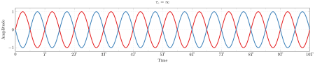
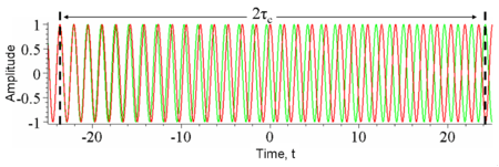
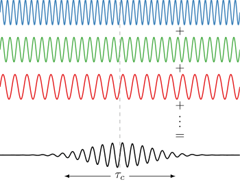
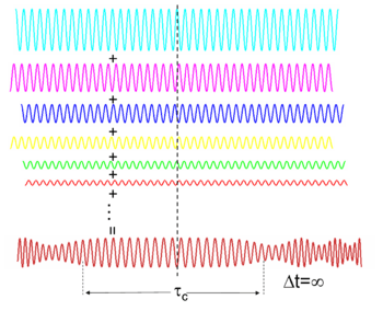
Figure 1: The amplitude of a single frequency wave as a function of time t (red) and a copy of the same wave delayed by τ (blue). The coherence time of the wave is infinite since it is perfectly correlated with itself for all delays τ.^[10]^:118

Figure 2: The amplitude of a wave whose phase drifts significantly in time τ_c as a function of time t (red) and a copy of the same wave delayed by 2τ_c(green). At any particular time t the wave can interfere perfectly with its delayed copy. But, since half the time the red and green waves are in phase and half the time out of phase, when averaged over t any interference disappears at this delay.

Temporal coherence is the measure of the average correlation between the value of a wave and itself delayed by τ, at any pair of times. Temporal coherence tells us how monochromatic a source is. In other words, it characterizes how well a wave can interfere with itself at a different time. The delay over which the phase or amplitude wanders by a significant amount (and hence the correlation decreases by significant amount) is defined as the coherence time τ_c. At a delay of τ=0 the degree of coherence is perfect, whereas it drops significantly as the delay passes τ=τ_c. The coherence length L_c is defined as the distance the wave travels in time τ_c.^[8]^{:560, 571–573}

One should be careful not to confuse the coherence time with the time duration of the signal, nor the coherence length with the coherence area (see below).

The relationship between coherence time and bandwidth

It can be shown that the larger the range of frequencies Δf a wave contains, the faster the wave decorrelates (and hence the smaller τ_c is). Thus there is a tradeoff:^[8]^{:358-359, 560}

\tau _{c}\Delta f\lesssim 1

Formally, this follows from the convolution theorem in mathematics, which relates the Fourier transform of the power spectrum (the intensity of each frequency) to its autocorrelation.^[8]^:572

Examples of temporal coherence

We consider four examples of temporal coherence.

A wave containing only a single frequency (monochromatic) is perfectly correlated with itself at all time delays, in accordance with the above relation. (See Figure 1)
Conversely, a wave whose phase drifts quickly will have a short coherence time. (See Figure 2)
Similarly, pulses (wave packets) of waves, which naturally have a broad range of frequencies, also have a short coherence time since the amplitude of the wave changes quickly. (See Figure 3)
Finally, white light, which has a very broad range of frequencies, is a wave which varies quickly in both amplitude and phase. Since it consequently has a very short coherence time (just 10 periods or so), it is often called incoherent.

Monochromatic sources are usually lasers; such high monochromaticity implies long coherence lengths (up to hundreds of meters). For example, a stabilized and monomode helium–neon laser can easily produce light with coherence lengths of 300 m.^[11] Not all lasers are monochromatic, however (e.g. for a mode-locked Ti-sapphire laser, Δλ ≈ 2 nm - 70 nm). LEDs are characterized by Δλ ≈ 50 nm, and tungsten filament lights exhibit Δλ ≈ 600 nm, so these sources have shorter coherence times than the most monochromatic lasers.

Holography requires light with a long coherence time. In contrast, optical coherence tomography uses light with a short coherence time.

Measurement of temporal coherence

Figure 3: The amplitude of a wavepacket whose amplitude changes significantly in time τ_c (red) and a copy of the same wave delayed by 2τ_c(green) plotted as a function of time t. At any particular time the red and green waves are uncorrelated; one oscillates while the other is constant and so there will be no interference at this delay. Another way of looking at this is the wavepackets are not overlapped in time and so at any particular time there is only one nonzero field so no interference can occur.

Figure 4: The time-averaged intensity (blue) detected at the output of an interferometer plotted as a function of delay τ for the example waves in Figures 2 and 3. As the delay is changed by half a period, the interference switches between constructive and destructive. The black lines indicate the interference envelope, which gives the degree of coherence. Although the waves in Figures 2 and 3 have different time durations, they have the same coherence time.

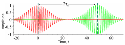
In optics, temporal coherence is measured in an interferometer such as the Michelson interferometer or Mach–Zehnder interferometer. In these devices, a wave is combined with a copy of itself that is delayed by time τ. A detector measures the time-averaged intensity of the light exiting the interferometer. The resulting interference visibility (e.g. see Figure 4) gives the temporal coherence at delay τ. Since for most natural light sources, the coherence time is much shorter than the time resolution of any detector, the detector itself does the time averaging. Consider the example shown in Figure 3. At a fixed delay, here 2τ_c, an infinitely fast detector would measure an intensity that fluctuates significantly over a time t equal to τ_c. In this case, to find the temporal coherence at 2τ_c, one would manually time-average the intensity.

Spatial coherence

In some systems, such as water waves or optics, wave-like states can extend over one or two dimensions. Spatial coherence describes the ability for two points in space, x₁ and x₂, in the extent of a wave to interfere, when averaged over time. More precisely, the spatial coherence is the cross-correlation between two points in a wave for all times. If a wave has only 1 value of amplitude over an infinite length, it is perfectly spatially coherent. The range of separation between the two points over which there is significant interference defines the diameter of the coherence area, A_c ^[12] (Coherence length, often a feature of a source, is usually an industrial term related to the coherence time of the source, not the coherence area in the medium.) A_c is the relevant type of coherence for the Young's double-slit interferometer. It is also used in optical imaging systems and particularly in various types of astronomy telescopes. Sometimes people also use "spatial coherence" to refer to the visibility when a wave-like state is combined with a spatially shifted copy of itself.

Examples of spatial coherence

Spatial coherence
Figure 5: A plane wave with an infinite coherence length.
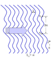Figure 6: A wave with a varying profile (wavefront) and infinite coherence length.
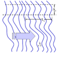Figure 7: A wave with a varying profile (wavefront) and finite coherence length.
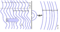Figure 8: A wave with finite coherence area is incident on a pinhole (small aperture). The wave will diffract out of the pinhole. Far from the pinhole the emerging spherical wavefronts are approximately flat. The coherence area is now infinite while the coherence length is unchanged.
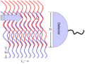Figure 9: A wave with infinite coherence area is combined with a spatially shifted copy of itself. Some sections in the wave interfere constructively and some will interfere destructively. Averaging over these sections, a detector with length D will measure reduced interference visibility. For example, a misaligned Mach–Zehnder interferometer will do this.

Consider a tungsten light-bulb filament. Different points in the filament emit light independently and have no fixed phase-relationship. In detail, at any point in time the profile of the emitted light is going to be distorted. The profile will change randomly over the coherence time $\tau _{c}$ . Since for a white-light source such as a light-bulb $\tau _{c}$ is small, the filament is considered a spatially incoherent source. In contrast, a radio antenna array, has large spatial coherence because antennas at opposite ends of the array emit with a fixed phase-relationship. Light waves produced by a laser often have high temporal and spatial coherence (though the degree of coherence depends strongly on the exact properties of the laser). Spatial coherence of laser beams also manifests itself as speckle patterns and diffraction fringes seen at the edges of shadow.

Holography requires temporally and spatially coherent light. Its inventor, Dennis Gabor, produced successful holograms more than ten years before lasers were invented. To produce coherent light he passed the monochromatic light from an emission line of a mercury-vapor lamp through a pinhole spatial filter.

In February 2011 it was reported that helium atoms, cooled to near absolute zero / Bose–Einstein condensate state, can be made to flow and behave as a coherent beam as occurs in a laser.^[13]^[14]

Spectral coherence

Figure 10: Waves of different frequencies interfere to form a localized pulse if they are coherent.

Figure 11: Spectrally incoherent light interferes to form continuous light with a randomly varying phase and amplitude

Waves of different frequencies (in light these are different colours) can interfere to form a pulse if they have a fixed relative phase-relationship (see Fourier transform). Conversely, if waves of different frequencies are not coherent, then, when combined, they create a wave that is continuous in time (e.g. white light or white noise). The temporal duration of the pulse $\Delta t$ is limited by the spectral bandwidth of the light $\Delta f$ according to:

\Delta f\Delta t\geq 1

which follows from the properties of the Fourier transform and results in Küpfmüller's uncertainty principle (for quantum particles it also results in the Heisenberg uncertainty principle).

If the phase depends linearly on the frequency (i.e. $\theta (f)\propto f$ ) then the pulse will have the minimum time duration for its bandwidth (a transform-limited pulse), otherwise it is chirped (see dispersion).

Measurement of spectral coherence

Measurement of the spectral coherence of light requires a nonlinear optical interferometer, such as an intensity optical correlator, frequency-resolved optical gating (FROG), or spectral phase interferometry for direct electric-field reconstruction (SPIDER).

Polarization and coherence

Light also has a polarization, which is the direction in which the electric field oscillates. Unpolarized light is composed of incoherent light waves with random polarization angles. The electric field of the unpolarized light wanders in every direction and changes in phase over the coherence time of the two light waves. An absorbing polarizer rotated to any angle will always transmit half the incident intensity when averaged over time.

If the electric field wanders by a smaller amount the light will be partially polarized so that at some angle, the polarizer will transmit more than half the intensity. If a wave is combined with an orthogonally polarized copy of itself delayed by less than the coherence time, partially polarized light is created.

The polarization of a light beam is represented by a vector in the Poincaré sphere. For polarized light the end of the vector lies on the surface of the sphere, whereas the vector has zero length for unpolarized light. The vector for partially polarized light lies within the sphere

Applications

Holography

Coherent superpositions of optical wave fields include holography. Holographic objects are used frequently in daily life in bank notes and credit cards.

Non-optical wave fields

Further applications concern the coherent superposition of non-optical wave fields. In quantum mechanics for example one considers a probability field, which is related to the wave function $\psi (\mathbf {r} )$ (interpretation: density of the probability amplitude). Here the applications concern, among others, the future technologies of quantum computing and the already available technology of quantum cryptography. Additionally the problems of the following subchapter are treated.

Quantum coherence

Further information: Quantum decoherence

In quantum mechanics, all objects have wave-like properties (see de Broglie waves). For instance, in Young's double-slit experiment electrons can be used in the place of light waves. Each electron's wave-function goes through both slits, and hence has two separate split-beams that contribute to the intensity pattern on a screen. According to standard wave theory ^[15] these two contributions give rise to an intensity pattern of bright bands due to constructive interference, interlaced with dark bands due to destructive interference, on a downstream screen. This ability to interfere and diffract is related to coherence (classical or quantum) of the waves produced at both slits. The association of an electron with a wave is unique to quantum theory.

When the incident beam is represented by a quantum pure state, the split beams downstream of the two slits are represented as a superposition of the pure states representing each split beam. The quantum description of imperfectly coherent paths is called a mixed state. A perfectly coherent state has a density matrix (also called the "statistical operator") that is a projection onto the pure coherent state and is equivalent to a wave function, while a mixed state is described by a classical probability distribution for the pure states that make up the mixture.

Macroscopic scale quantum coherence leads to novel phenomena, the so-called macroscopic quantum phenomena. For instance, the laser, superconductivity and superfluidity are examples of highly coherent quantum systems whose effects are evident at the macroscopic scale. The macroscopic quantum coherence (Off-Diagonal Long-Range Order, ODLRO)^[16]^[17] for superfluidity, and laser light, is related to first-order (1-body) coherence/ODLRO, while superconductivity is related to second-order coherence/ODLRO. (For fermions, such as electrons, only even orders of coherence/ODLRO are possible.) For bosons, a Bose–Einstein condensate is an example of a system exhibiting macroscopic quantum coherence through a multiple occupied single-particle state.

Regarding the occurrence of quantum coherence at a macroscopic level, it is interesting to note that the classical electromagnetic field exhibits macroscopic quantum coherence. The most obvious example is the carrier signal for radio and TV. They satisfy Glauber's quantum description of coherence.

Recently M.B. Plenio and co-workers constructed an operational formulation of Quantum coherence as a resource theory. They introduced coherence monotones analogous to the entanglement monotones. ^[18]

References

↑ Hecht (1998). Optics (3rd ed.). Addison Wesley Longman. pp. 554–574. ISBN 0-201-83887-7.
↑ Shin. K, Hammond. J. Fundamentals of signal processing for sound and vibration engineers. John Wiley & Sons, 2008.
↑ Rolf G. Winter; Aephraim M. Steinberg (2008). "Coherence". AccessScience. McGraw-Hill.
↑ M.Born; E. Wolf (1999). Principles of Optics (7th ed.). Cambridge University Press. ISBN 978-0-521-64222-4.
↑ Loudon, Rodney (2000). The Quantum Theory of Light. Oxford University Press. ISBN 0-19-850177-3.
↑ Leonard Mandel; Emil Wolf (1995). Optical Coherence and Quantum Optics. Cambridge University Press. ISBN 0-521-41711-2.
↑ Arvind Marathay (1982). Elements of Optical Coherence Theory. John Wiley & Sons. ISBN 0-471-56789-2.
1 2 3 4 Hecht, Eugene (2002), Optics (4th ed.), United States of America: Addison Wesley, ISBN 0-8053-8566-5
↑ Peng, J.-L.; Liu, T.-A.; Shu, R.-H. (2008). "Optical frequency counter based on two mode-locked fiber laser combs". Applied Physics B. 92 (4): 513. Bibcode:2008ApPhB..92..513P. doi:10.1007/s00340-008-3111-6.
↑ Christopher Gerry; Peter Knight (2005). Introductory Quantum Optics. Cambridge University Press. ISBN 978-0-521-52735-4.
↑ Saleh, Teich. Fundamentals of Photonics. Wiley.
↑ Goodman (1985). Statistical Optics (1st ed.). Wiley-Interscience. pp. 210,221. ISBN 0-471-01502-4.
↑ Hodgman, S. S.; Dall, R. G.; Manning, A. G.; Baldwin, K. G. H.; Truscott, A. G. (2011). "Direct Measurement of Long-Range Third-Order Coherence in Bose-Einstein Condensates". Science. 331 (6020): 1046–1049. Bibcode:2011Sci...331.1046H. doi:10.1126/science.1198481. PMID 21350171.
↑ Pincock, S. (25 February 2011). "Cool laser makes atoms march in time". ABC Science. ABC News Online. Retrieved 2011-03-02.
↑ A. P. French (2003). Vibrations and Waves. Norton. ISBN 0-393-09936-9.
↑ Penrose, O.; Onsager, L. (1956). "Bose-Einstein Condensation and Liquid Helium". Phys. Rev. 104: 576.
↑ Yang, C.N. (1962). "Concept of Off-Diagonal Long-Range Order and the Quantum Phases of Liquid He and of Superconductors". Rev. Mod. Phys. 34: 694.
↑ Baumgratz, T.; Cramer, M.; Plenio, M.B. (2014). "Quantifying Coherence". Phys. Rev. Lett. 113: 140401.

External links

"Dr. SkySkull". "Optics basics: Coherence". Skulls in the Stars.

This article is issued from Wikipedia - version of the 11/27/2016. The text is available under the Creative Commons Attribution/Share Alike but additional terms may apply for the media files.