Simultaneous perturbation stochastic approximation
Simultaneous perturbation stochastic approximation (SPSA) is an algorithmic method for optimizing systems with multiple unknown parameters. It is a type of stochastic approximation algorithm. As an optimization method, it is appropriately suited to large-scale population models, adaptive modeling, simulation optimization, and atmospheric modeling. Many examples are presented at the SPSA website http://www.jhuapl.edu/SPSA. A comprehensive recent book on the subject is Bhatnagar et al. (2013). An early paper on the subject is Spall (1987) and the foundational paper providing the key theory and justification is Spall (1992).
SPSA is a descent method capable of finding global minima, sharing this property with other methods as simulated annealing. Its main feature is the gradient approximation that requires only two measurements of the objective function, regardless of the dimension of the optimization problem. Recall that we want to find the optimal control  with loss
function
with loss
function  :
:
Both Finite Differences Stochastic Approximation (FDSA) and SPSA use the same iterative process:
where  represents the
  iterate,
  is the estimate of the gradient of the objective function
  evaluated at
  , and
, and  is a positive number sequence converging to 0. If
  is a p-dimensional vector, the
  component of the symmetric finite difference gradient estimator is:
- FD:
1 ≤i ≤p, where  is the unit vector with a 1 in the
place, and
is the unit vector with a 1 in the
place, and  is a small positive number that decreases with n. With this method, 2p evaluations of J for each
  are needed. Clearly, when p is large, this estimator loses efficiency.
Let now  be a random perturbation vector. The component of the stochastic perturbation gradient estimator is:
- SP:
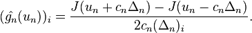
Remark that FD perturbs only one direction at a time, while the SP estimator disturbs all directions at the same time (the numerator is identical in all p components). The number of loss function measurements needed in the SPSA method for each is always 2, independent of the dimension p. Thus, SPSA uses p times fewer function evaluations than FDSA, which makes it a lot more efficient.
Simple experiments with p=2 showed that SPSA converges in the same number of iterations as FDSA. The latter follows approximately the steepest descent direction, behaving like the gradient method. On the other hand, SPSA, with the random search direction, does not follow exactly the gradient path. In average though, it tracks it nearly because the gradient approximation is an almost unbiased estimator of the gradient, as shown in the following lemma.
Convergence lemma
Denote by
![b_n = E[\hat{g}_n|u_n] -\nabla J(u_n)](../I/m/702bf36a679199295c48780f36558b7a.png)
the bias in the estimator  . Assume that
  are all mutually independent with zero-mean, bounded second
moments, and
are all mutually independent with zero-mean, bounded second
moments, and 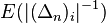 uniformly bounded. Then
  →0 w.p. 1.
Sketch of the proof
The main idea is to use conditioning on to express ![E[(\hat{g}_n)_i]](../I/m/404c64418da8c1f2a19622f5b021baf4.png) and then to use a second order Taylor expansion of
and then to use a second order Taylor expansion of 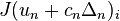 and
and  . After algebraic manipulations using the zero mean and the independence of , we get
![E[(\hat{g}_n)_i]=(g_n)_i + O(c_n^2)](../I/m/841cf800cd9a4210f1591a0aef687893.png)
The result follows from the hypothesis that →0.
Next we resume some of the hypotheses under which  converges in probability to the set of global minima of . The efficiency of
the method depends on the shape of , the values of the parameters
converges in probability to the set of global minima of . The efficiency of
the method depends on the shape of , the values of the parameters  and
and  and the distribution of the perturbation terms
  . First, the algorithm parameters must satisfy the
following conditions:
. First, the algorithm parameters must satisfy the
following conditions:
-
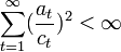
 >0, →0 when t→∝ and
  . A good choice would be
  a>0;
a>0; -
 , where c>0,
 ![\gamma \in \left[\frac{1}{6},\frac{1}{2}\right]](../I/m/f4e7fb5916979d55726d388796f23039.png) ;
; -
-
 must be mutually independent zero-mean random variables, symmetrically distributed about zero, with
  . The inverse first and second moments of the must be finite.
A good choice for is the Rademacher distribution, i.e. Bernoulli +-1 with probability 0.5. Other choices are possible too, but note that the uniform and normal distributions cannot be used because they do not satisfy the finite inverse moment conditions.
The loss function J(u) must be thrice continuously differentiable and the individual elements of the third derivative must be bounded:  . Also, |J(u)|→∝ as u→∝.
In addition,  must be Lipschitz continuous, bounded and the ODE
  must have a unique solution for each initial condition.
Under these conditions and a few others,
must have a unique solution for each initial condition.
Under these conditions and a few others,  converges in probability to the set of global minima of J(u) (see Maryak and Chin, 2008).
References
- Bhatnagar, S., Prasad, H. L., and Prashanth, L. A. (2013), Stochastic Recursive Algorithms for Optimization: Simultaneous Perturbation Methods, Springer .
- Hirokami, T., Maeda, Y., Tsukada, H. (2006) "Parameter estimation using simultaneous perturbation stochastic approximation", Electrical Engineering in Japan, 154 (2), 30–3
- Maryak, J.L., and Chin, D.C. (2008), "Global Random Optimization by Simultaneous Perturbation Stochastic Approximation," IEEE Transactions on Automatic Control, vol. 53, pp. 780-783.
- Spall, J. C. (1987), “A Stochastic Approximation Technique for Generating Maximum Likelihood Parameter Estimates,” Proceedings of the American Control Conference, Minneapolis, MN, June 1987, pp. 1161–1167.
- Spall, J. C. (1992), “Multivariate Stochastic Approximation Using a Simultaneous Perturbation Gradient Approximation,” IEEE Transactions on Automatic Control, vol. 37(3), pp. 332–341.
- Spall, J.C. (1998). "Overview of the Simultaneous Perturbation Method for Efficient Optimization" 2. Johns Hopkins APL Technical Digest, 19(4), 482–492.
- Spall, J.C. (2003) Introduction to Stochastic Search and Optimization: Estimation, Simulation, and Control, Wiley. ISBN 0-471-33052-3 (Chapter 7)