Shapley–Folkman lemma
The Shapley–Folkman lemma is a result in convex geometry with applications in mathematical economics that describes the Minkowski addition of sets in a vector space. Minkowski addition is defined as the addition of the sets' members: for example, adding the set consisting of the integers zero and one to itself yields the set consisting of zero, one, and two:
- {0, 1} + {0, 1} = {0 + 0, 0 + 1, 1 + 0, 1 + 1} = {0, 1, 2}.
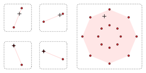
The Shapley–Folkman lemma and related results provide an affirmative answer to the question, "Is the sum of many sets close to being convex?"[2] A set is defined to be convex if every line segment joining two of its points is a subset in the set: For example, the solid disk is a convex set but the circle is not, because the line segment joining two distinct points is not a subset of the circle. The Shapley–Folkman lemma suggests that if the number of summed sets exceeds the dimension of the vector space, then their Minkowski sum is approximately convex.[1]


The Shapley–Folkman lemma was introduced as a step in the proof of the Shapley–Folkman theorem, which states an upper bound on the distance between the Minkowski sum and its convex hull. The convex hull of a set Q is the smallest convex set that contains Q. This distance is zero if and only if the sum is convex. The theorem's bound on the distance depends on the dimension D and on the shapes of the summand-sets, but not on the number of summand-sets N, when N > D. The shapes of a subcollection of only D summand-sets determine the bound on the distance between the Minkowski average of N sets
- 1⁄N (Q1 + Q2 + ... + QN)
and its convex hull. As N increases to infinity, the bound decreases to zero (for summand-sets of uniformly bounded size).[3] The Shapley–Folkman theorem's upper bound was decreased by Starr's corollary (alternatively, the Shapley–Folkman–Starr theorem).
The lemma of Lloyd Shapley and Jon Folkman was first published by the economist Ross M. Starr, who was investigating the existence of economic equilibria while studying with Kenneth Arrow.[1] In his paper, Starr studied a convexified economy, in which non-convex sets were replaced by their convex hulls; Starr proved that the convexified economy has equilibria that are closely approximated by "quasi-equilibria" of the original economy; moreover, he proved that every quasi-equilibrium has many of the optimal properties of true equilibria, which are proved to exist for convex economies. Following Starr's 1969 paper, the Shapley–Folkman–Starr results have been widely used to show that central results of (convex) economic theory are good approximations to large economies with non-convexities; for example, quasi-equilibria closely approximate equilibria of a convexified economy. "The derivation of these results in general form has been one of the major achievements of postwar economic theory", wrote Roger Guesnerie.[4] The topic of non-convex sets in economics has been studied by many Nobel laureates, besides Lloyd Shapley who won the prize in 2012: Arrow (1972), Robert Aumann (2005), Gérard Debreu (1983), Tjalling Koopmans (1975), Paul Krugman (2008), and Paul Samuelson (1970); the complementary topic of convex sets in economics has been emphasized by these laureates, along with Leonid Hurwicz, Leonid Kantorovich (1975), and Robert Solow (1987).
The Shapley–Folkman lemma has applications also in optimization and probability theory.[3] In optimization theory, the Shapley–Folkman lemma has been used to explain the successful solution of minimization problems that are sums of many functions.[5][6] The Shapley–Folkman lemma has also been used in proofs of the "law of averages" for random sets, a theorem that had been proved for only convex sets.[7]
Introductory example
For example, the subset of the integers {0, 1, 2} is contained in the interval of real numbers [0, 2], which is convex. The Shapley–Folkman lemma implies that every point in [0, 2] is the sum of an integer from {0, 1} and a real number from [0, 1].[8]
The distance between the convex interval [0, 2] and the non-convex set {0, 1, 2} equals one-half
- 1/2 = |1 − 1/2| = |0 − 1/2| = |2 − 3/2| = |1 − 3/2|.
However, the distance between the average Minkowski sum
- 1/2 ( {0, 1} + {0, 1} ) = {0, 1/2, 1}
and its convex hull [0, 1] is only 1/4, which is half the distance (1/2) between its summand {0, 1} and [0, 1]. As more sets are added together, the average of their sum "fills out" its convex hull: The maximum distance between the average and its convex hull approaches zero as the average includes more summands.[8]
Preliminaries
The Shapley–Folkman lemma depends upon the following definitions and results from convex geometry.
Real vector spaces
A real vector space of two dimensions can be given a Cartesian coordinate system in which every point is identified by an ordered pair of real numbers, called "coordinates", which are conventionally denoted by x and y. Two points in the Cartesian plane can be added coordinate-wise
- (x1, y1) + (x2, y2) = (x1+x2, y1+y2);
further, a point can be multiplied by each real number λ coordinate-wise
- λ (x, y) = (λx, λy).
More generally, any real vector space of (finite) dimension D can be viewed as the set of all D-tuples of D real numbers { (v1, v2, . . . , vD) } on which two operations are defined: vector addition and multiplication by a real number. For finite-dimensional vector spaces, the operations of vector addition and real-number multiplication can each be defined coordinate-wise, following the example of the Cartesian plane.[9]
Convex sets
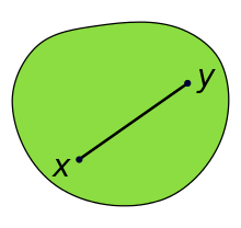
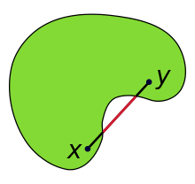
In a real vector space, a non-empty set Q is defined to be convex if, for each pair of its points, every point on the line segment that joins them is a subset of Q. For example, a solid disk is convex but a circle is not, because it does not contain a line segment joining its points ; the non-convex set of three integers {0, 1, 2} is contained in the interval [0, 2], which is convex. For example, a solid cube is convex; however, anything that is hollow or dented, for example, a crescent shape, is non-convex. The empty set is convex, either by definition[10] or vacuously, depending on the author.
More formally, a set Q is convex if, for all points v0 and v1 in Q and for every real number λ in the unit interval [0,1], the point
- (1 − λ) v0 + λv1
is a member of Q.
By mathematical induction, a set Q is convex if and only if every convex combination of members of Q also belongs to Q. By definition, a convex combination of an indexed subset {v0, v1, . . . , vD} of a vector space is any weighted average λ0v0 + λ1v1 + . . . + λDvD, for some indexed set of non-negative real numbers {λd} satisfying the equation λ0 + λ1 + . . . + λD = 1.[11]
The definition of a convex set implies that the intersection of two convex sets is a convex set. More generally, the intersection of a family of convex sets is a convex set. In particular, the intersection of two disjoint sets is the empty set, which is convex.[10]
Convex hull
For every subset Q of a real vector space, its convex hull Conv(Q) is the minimal convex set that contains Q. Thus Conv(Q) is the intersection of all the convex sets that cover Q. The convex hull of a set can be equivalently defined to be the set of all convex combinations of points in Q.[12] For example, the convex hull of the set of integers {0,1} is the closed interval of real numbers [0,1], which contains the integer end-points.[8] The convex hull of the unit circle is the closed unit disk, which contains the unit circle.
Minkowski addition
![Three squares are shown in the non-negative quadrant of the Cartesian plane. The square Q1=[0,1]×[0,1] is green. The square Q2=[1,2]×[1,2] is brown, and it sits inside the turquoise square Q1+Q2=[1,3]×[1,3].](../I/m/Minkowski_sum.png)
In a real vector space, the Minkowski sum of two (non-empty) sets Q1 and Q2 is defined to be the set Q1 + Q2 formed by the addition of vectors element-wise from the summand sets
- Q1 + Q2 = { q1 + q2 : q1 ∈ Q1 and q2 ∈ Q2 }.[13]
For example
- {0, 1} + {0, 1} = {0+0, 0+1, 1+0, 1+1} = {0, 1, 2}.[8]
By the principle of mathematical induction, the Minkowski sum of a finite family of (non-empty) sets
- {Qn : Qn ≠ Ø and 1 ≤ n ≤ N }
is the set formed by element-wise addition of vectors
- ∑ Qn = {∑ qn : qn ∈ Qn}.[14]
Convex hulls of Minkowski sums
Minkowski addition behaves well with respect to "convexification"—the operation of taking convex hulls. Specifically, for all subsets Q1 and Q2 of a real vector space, the convex hull of their Minkowski sum is the Minkowski sum of their convex hulls. That is,
- Conv( Q1 + Q2 ) = Conv( Q1 ) + Conv( Q2 ).
This result holds more generally, as a consequence of the principle of mathematical induction. For each finite collection of sets,
Statements
The preceding identity Conv( ∑ Qn ) = ∑ Conv( Qn ) implies that if a point x lies in the convex hull of the Minkowski sum of N sets
- x ∈ Conv( ∑ Qn )
then x lies in the sum of the convex hulls of the summand-sets
- x ∈ ∑ Conv( Qn ).
By the definition of Minkowski addition, this last expression means that x = ∑ qn for some selection of points qn in the convex hulls of the summand-sets, that is, where each qn ∈ Conv(Qn). In this representation, the selection of the summand-points qn depends on the chosen sum-point x.
Lemma of Shapley and Folkman
.jpg)
For this representation of the point x, the Shapley–Folkman lemma states that if the dimension D is less than the number of summands
- D < N
then convexification is needed for only D summand-sets, whose choice depends on x: The point has a representation

where qd belongs to the convex hull of Qd for D (or fewer) summand-sets and qn belongs to Qn itself for the remaining sets. That is,

for some re-indexing of the summand sets; this re-indexing depends on the particular point x being represented.[17]
The Shapley–Folkman lemma implies, for example, that every point in [0, 2] is the sum of an integer from {0, 1} and a real number from [0, 1].[8]
Dimension of a real vector space
Conversely, the Shapley–Folkman lemma characterizes the dimension of finite-dimensional, real vector spaces. That is, if a vector space obeys the Shapley–Folkman lemma for a natural number D, and for no number less than D, then its dimension is exactly D;[18] the Shapley–Folkman lemma holds for only finite-dimensional vector spaces.[19]
Shapley–Folkman theorem and Starr's corollary

Shapley and Folkman used their lemma to prove their theorem, which bounds the distance between a Minkowski sum and its convex hull, the "convexified" sum:
- The Shapley–Folkman theorem states that the squared Euclidean distance from any point in the convexified sum Conv( ∑ Qn ) to the original (unconvexified) sum ∑ Qn is bounded by the sum of the squares of the D largest circumradii of the sets Qn (the radii of the smallest spheres enclosing these sets).[20] This bound is independent of the number of summand-sets N (if N > D).[21]
The Shapley–Folkman theorem states a bound on the distance between the Minkowski sum and its convex hull; this distance is zero if and only if the sum is convex. Their bound on the distance depends on the dimension D and on the shapes of the summand-sets, but not on the number of summand-sets N, when N > D.[3]
The circumradius often exceeds (and cannot be less than) the inner radius:[22]
- The inner radius of a set Qn is defined to be the smallest number r such that, for any point q in the convex hull of Qn, there is a sphere of radius r that contains a subset of Qn whose convex hull contains q.
Starr used the inner radius to reduce the upper bound stated in the Shapley–Folkman theorem:
- Starr's corollary to the Shapley–Folkman theorem states that the squared Euclidean distance from any point x in the convexified sum Conv( ∑ Qn ) to the original (unconvexified) sum ∑ Qn is bounded by the sum of the squares of the D largest inner-radii of the sets Qn.[22][23]
Starr's corollary states an upper bound on the Euclidean distance between the Minkowski sum of N sets and the convex hull of the Minkowski sum; this distance between the sum and its convex hull is a measurement of the non-convexity of the set. For simplicity, this distance is called the "non-convexity" of the set (with respect to Starr's measurement). Thus, Starr's bound on the non-convexity of the sum depends on only the D largest inner radii of the summand-sets; however, Starr's bound does not depend on the number of summand-sets N, when N > D. For example, the distance between the convex interval [0, 2] and the non-convex set {0, 1, 2} equals one-half
- 1/2 = |1 − 1/2| = |0 − 1/2| = |2 − 3/2| = |1 − 3/2|.
Thus, Starr's bound on the non-convexity of the average
- 1⁄N ∑ Qn
decreases as the number of summands N increases. For example, the distance between the averaged set
- 1/2 ( {0, 1} + {0, 1} ) = {0, 1/2, 1}
and its convex hull [0, 1] is only 1/4, which is half the distance (1/2) between its summand {0, 1} and [0, 1]. The shapes of a subcollection of only D summand-sets determine the bound on the distance between the average set and its convex hull; thus, as the number of summands increases to infinity, the bound decreases to zero (for summand-sets of uniformly bounded size).[3] In fact, Starr's bound on the non-convexity of this average set decreases to zero as the number of summands N increases to infinity (when the inner radii of all the summands are bounded by the same number).[3]
Proofs and computations
The original proof of the Shapley–Folkman lemma established only the existence of the representation, but did not provide an algorithm for computing the representation: Similar proofs have been given by Arrow and Hahn,[24] Cassels,[25] and Schneider,[26] among others. An abstract and elegant proof by Ekeland has been extended by Artstein.[27][28] Different proofs have appeared in unpublished papers, also.[2][29] In 1981, Starr published an iterative method for computing a representation of a given sum-point; however, his computational proof provides a weaker bound than does the original result.[30] An elementary proof of the Shapley–Folkman lemma in finite-dimensional space can be found in the book by Bertsekas[31] together with applications in estimating the duality gap in separable optimization problems and zero-sum games.
Applications
The Shapley–Folkman lemma enables researchers to extend results for Minkowski sums of convex sets to sums of general sets, which need not be convex. Such sums of sets arise in economics, in mathematical optimization, and in probability theory; in each of these three mathematical sciences, non-convexity is an important feature of applications.
Economics
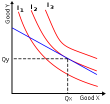
In economics, a consumer's preferences are defined over all "baskets" of goods. Each basket is represented as a non-negative vector, whose coordinates represent the quantities of the goods. On this set of baskets, an indifference curve is defined for each consumer; a consumer's indifference curve contains all the baskets of commodities that the consumer regards as equivalent: That is, for every pair of baskets on the same indifference curve, the consumer does not prefer one basket over another. Through each basket of commodities passes one indifference curve. A consumer's preference set (relative to an indifference curve) is the union of the indifference curve and all the commodity baskets that the consumer prefers over the indifference curve. A consumer's preferences are convex if all such preference sets are convex.[32]
An optimal basket of goods occurs where the budget-line supports a consumer's preference set, as shown in the diagram. This means that an optimal basket is on the highest possible indifference curve given the budget-line, which is defined in terms of a price vector and the consumer's income (endowment vector). Thus, the set of optimal baskets is a function of the prices, and this function is called the consumer's demand. If the preference set is convex, then at every price the consumer's demand is a convex set, for example, a unique optimal basket or a line-segment of baskets.[33]
Non-convex preferences
However, if a preference set is non-convex, then some prices determine a budget-line that supports two separate optimal-baskets. For example, we can imagine that, for zoos, a lion costs as much as an eagle, and further that a zoo's budget suffices for one eagle or one lion. We can suppose also that a zoo-keeper views either animal as equally valuable. In this case, the zoo would purchase either one lion or one eagle. Of course, a contemporary zoo-keeper does not want to purchase half of an eagle and half of a lion (or a griffin)! Thus, the zoo-keeper's preferences are non-convex: The zoo-keeper prefers having either animal to having any strictly convex combination of both.[34]
When the consumer's preference set is non-convex, then (for some prices) the consumer's demand is not connected; a disconnected demand implies some discontinuous behavior by the consumer, as discussed by Harold Hotelling:
If indifference curves for purchases be thought of as possessing a wavy character, convex to the origin in some regions and concave in others, we are forced to the conclusion that it is only the portions convex to the origin that can be regarded as possessing any importance, since the others are essentially unobservable. They can be detected only by the discontinuities that may occur in demand with variation in price-ratios, leading to an abrupt jumping of a point of tangency across a chasm when the straight line is rotated. But, while such discontinuities may reveal the existence of chasms, they can never measure their depth. The concave portions of the indifference curves and their many-dimensional generalizations, if they exist, must forever remain in unmeasurable obscurity.[35]
The difficulties of studying non-convex preferences were emphasized by Herman Wold[36] and again by Paul Samuelson, who wrote that non-convexities are "shrouded in eternal darkness ...",[37] according to Diewert.[38]
Nonetheless, non-convex preferences were illuminated from 1959 to 1961 by a sequence of papers in The Journal of Political Economy (JPE). The main contributors were Farrell,[39] Bator,[40] Koopmans,[41] and Rothenberg.[42] In particular, Rothenberg's paper discussed the approximate convexity of sums of non-convex sets.[43] These JPE-papers stimulated a paper by Lloyd Shapley and Martin Shubik, which considered convexified consumer-preferences and introduced the concept of an "approximate equilibrium".[44] The JPE-papers and the Shapley–Shubik paper influenced another notion of "quasi-equilibria", due to Robert Aumann.[45][46]
Starr's 1969 paper and contemporary economics

Previous publications on non-convexity and economics were collected in an annotated bibliography by Kenneth Arrow. He gave the bibliography to Starr, who was then an undergraduate enrolled in Arrow's (graduate) advanced mathematical-economics course.[47] In his term-paper, Starr studied the general equilibria of an artificial economy in which non-convex preferences were replaced by their convex hulls. In the convexified economy, at each price, the aggregate demand was the sum of convex hulls of the consumers' demands. Starr's ideas interested the mathematicians Lloyd Shapley and Jon Folkman, who proved their eponymous lemma and theorem in "private correspondence", which was reported by Starr's published paper of 1969.[1]
In his 1969 publication, Starr applied the Shapley–Folkman–Starr theorem. Starr proved that the "convexified" economy has general equilibria that can be closely approximated by "quasi-equilibria" of the original economy, when the number of agents exceeds the dimension of the goods: Concretely, Starr proved that there exists at least one quasi-equilibrium of prices popt with the following properties:
- For each quasi-equilibrium's prices popt, all consumers can choose optimal baskets (maximally preferred and meeting their budget constraints).
- At quasi-equilibrium prices popt in the convexified economy, every good's market is in equilibrium: Its supply equals its demand.
- For each quasi-equilibrium, the prices "nearly clear" the markets for the original economy: an upper bound on the distance between the set of equilibria of the "convexified" economy and the set of quasi-equilibria of the original economy followed from Starr's corollary to the Shapley–Folkman theorem.[48]
Starr established that
"in the aggregate, the discrepancy between an allocation in the fictitious economy generated by [taking the convex hulls of all of the consumption and production sets] and some allocation in the real economy is bounded in a way that is independent of the number of economic agents. Therefore, the average agent experiences a deviation from intended actions that vanishes in significance as the number of agents goes to infinity".[49]
Following Starr's 1969 paper, the Shapley–Folkman–Starr results have been widely used in economic theory. Roger Guesnerie summarized their economic implications: "Some key results obtained under the convexity assumption remain (approximately) relevant in circumstances where convexity fails. For example, in economies with a large consumption side, preference nonconvexities do not destroy the standard results".[50] "The derivation of these results in general form has been one of the major achievements of postwar economic theory", wrote Guesnerie.[4] The topic of non-convex sets in economics has been studied by many Nobel laureates: Arrow (1972), Robert Aumann (2005), Gérard Debreu (1983), Tjalling Koopmans (1975), Paul Krugman (2008), and Paul Samuelson (1970); the complementary topic of convex sets in economics has been emphasized by these laureates, along with Leonid Hurwicz, Leonid Kantorovich (1975), and Robert Solow (1987).[51] The Shapley–Folkman–Starr results have been featured in the economics literature: in microeconomics,[52] in general-equilibrium theory,[53][54] in public economics[55] (including market failures),[56] as well as in game theory,[57] in mathematical economics,[58] and in applied mathematics (for economists).[59][60] The Shapley–Folkman–Starr results have also influenced economics research using measure and integration theory.[61]
Mathematical optimization
The Shapley–Folkman lemma has been used to explain why large minimization problems with non-convexities can be nearly solved (with iterative methods whose convergence proofs are stated for only convex problems). The Shapley–Folkman lemma has encouraged the use of methods of convex minimization on other applications with sums of many functions.[62]
Preliminaries of optimization theory
Nonlinear optimization relies on the following definitions for functions:
- Graph(f) = { (x, f(x) ) }
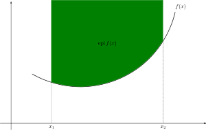
- The epigraph of a real-valued function f is the set of points above the graph
- Epi(f) = { (x, u) : f(x) ≤ u }.
- A real-valued function is defined to be a convex function if its epigraph is a convex set.[63]
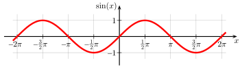
For example, the quadratic function f(x) = x2 is convex, as is the absolute value function g(x) = |x|. However, the sine function (pictured) is non-convex on the interval (0, π).
Additive optimization problems
In many optimization problems, the objective function f is separable: that is, f is the sum of many summand-functions, each of which has its own argument:
- f(x) = f( (x1, ..., xN) ) = ∑ fn(xn).
For example, problems of linear optimization are separable. Given a separable problem with an optimal solution, we fix an optimal solution
- xmin = (x1, ..., xN)min
with the minimum value f(xmin). For this separable problem, we also consider an optimal solution (xmin, f(xmin) ) to the "convexified problem", where convex hulls are taken of the graphs of the summand functions. Such an optimal solution is the limit of a sequence of points in the convexified problem
Of course, the given optimal-point is a sum of points in the graphs of the original summands and of a small number of convexified summands, by the Shapley–Folkman lemma.
This analysis was published by Ivar Ekeland in 1974 to explain the apparent convexity of separable problems with many summands, despite the non-convexity of the summand problems. In 1973, the young mathematician Claude Lemaréchal was surprised by his success with convex minimization methods on problems that were known to be non-convex; for minimizing nonlinear problems, a solution of the dual problem problem need not provide useful information for solving the primal problem, unless the primal problem be convex and satisfy a constraint qualification. Lemaréchal's problem was additively separable, and each summand function was non-convex; nonetheless, a solution to the dual problem provided a close approximation to the primal problem's optimal value.[65][5][66] Ekeland's analysis explained the success of methods of convex minimization on large and separable problems, despite the non-convexities of the summand functions. Ekeland and later authors argued that additive separability produced an approximately convex aggregate problem, even though the summand functions were non-convex. The crucial step in these publications is the use of the Shapley–Folkman lemma.[5][66][67] The Shapley–Folkman lemma has encouraged the use of methods of convex minimization on other applications with sums of many functions.[5][6][59][62]
Probability and measure theory
Convex sets are often studied with probability theory. Each point in the convex hull of a (non-empty) subset Q of a finite-dimensional space is the expected value of a simple random vector that takes its values in Q, as a consequence of Carathéodory's lemma. Thus, for a non-empty set Q, the collection of the expected values of the simple, Q-valued random vectors equals Q's convex hull; this equality implies that the Shapley–Folkman–Starr results are useful in probability theory.[68] In the other direction, probability theory provides tools to examine convex sets generally and the Shapley–Folkman–Starr results specifically.[69] The Shapley–Folkman–Starr results have been widely used in the probabilistic theory of random sets,[70] for example, to prove a law of large numbers,[7][71] a central limit theorem,[71][72] and a large-deviations principle.[73] These proofs of probabilistic limit theorems used the Shapley–Folkman–Starr results to avoid the assumption that all the random sets be convex.
A probability measure is a finite measure, and the Shapley–Folkman lemma has applications in non-probabilistic measure theory, such as the theories of volume and of vector measures. The Shapley–Folkman lemma enables a refinement of the Brunn–Minkowski inequality, which bounds the volume of sums in terms of the volumes of their summand-sets.[74] The volume of a set is defined in terms of the Lebesgue measure, which is defined on subsets of Euclidean space. In advanced measure-theory, the Shapley–Folkman lemma has been used to prove Lyapunov's theorem, which states that the range of a vector measure is convex.[75] Here, the traditional term "range" (alternatively, "image") is the set of values produced by the function. A vector measure is a vector-valued generalization of a measure; for example, if p1 and p2 are probability measures defined on the same measurable space, then the product function p1 p2 is a vector measure, where p1 p2 is defined for every event ω by
- (p1 p2)(ω)=(p1(ω), p2(ω)).
Lyapunov's theorem has been used in economics,[45][76] in ("bang-bang") control theory, and in statistical theory.[77] Lyapunov's theorem has been called a continuous counterpart of the Shapley–Folkman lemma,[3] which has itself been called a discrete analogue of Lyapunov's theorem.[78]
Notes
- 1 2 3 4 5 Starr (1969)
- 1 2 Howe (1979, p. 1): Howe, Roger (3 November 1979), On the tendency toward convexity of the vector sum of sets (PDF), Cowles Foundation discussion papers, 538, Box 2125 Yale Station, New Haven,CT 06520: Cowles Foundation for Research in Economics, Yale University, retrieved 1 January 2011
- 1 2 3 4 5 6 Starr (2008)
- 1 2 Guesnerie (1989, p. 138)
- 1 2 3 4 5 (Ekeland 1999, pp. 357–359): Published in the first English edition of 1976, Ekeland's appendix proves the Shapley–Folkman lemma, also acknowledging Lemaréchal's experiments on page 373.
- 1 2 Bertsekas (1996, pp. 364–381) acknowledging Ekeland (1999) on page 374 and Aubin & Ekeland (1976) on page 381:
Bertsekas, Dimitri P. (1996). "5.6 Large scale separable integer programming problems and the exponential method of multipliers". Constrained optimization and Lagrange multiplier methods (Reprint of (1982) Academic Press ed.). Belmont, MA: Athena Scientific. pp. xiii+395. ISBN 1-886529-04-3. MR 690767.
Bertsekas (1996, pp. 364–381) describes an application of Lagrangian dual methods to the scheduling of electrical power plants ("unit commitment problems"), where non-convexity appears because of integer constraints:
Bertsekas, Dimitri P.; Lauer, Gregory S.; Sandell, Nils R., Jr.; Posbergh, Thomas A. (January 1983). "Optimal short-term scheduling of large-scale power systems" (PDF). IEEE Transactions on Automatic Control. AC-28 (Proceedings of 1981 IEEE Conference on Decision and Control, San Diego, CA, December 1981, pp. 432–443): 1–11. Retrieved 2 February 2011.
- 1 2 Artstein & Vitale (1975, pp. 881–882): Artstein, Zvi; Vitale, Richard A. (1975), "A strong law of large numbers for random compact sets", The Annals of Probability, 3 (5): 879–882, doi:10.1214/aop/1176996275, JSTOR 2959130, MR 385966, Zbl 0313.60012, PE euclid.ss/1176996275
- 1 2 3 4 5 Carter (2001, p. 94)
- ↑ Arrow & Hahn (1980, p. 375)
- 1 2 Rockafellar (1997, p. 10)
- ↑ Arrow & Hahn (1980, p. 376), Rockafellar (1997, pp. 10–11), and Green & Heller (1981, p. 37)
- ↑ Arrow & Hahn (1980, p. 385) and Rockafellar (1997, pp. 11–12)
- ↑ Schneider (1993, p. xi) and Rockafellar (1997, p. 16)
- ↑ Rockafellar (1997, p. 17) and Starr (1997, p. 78)
- ↑ Schneider (1993, pp. 2–3)
- ↑ Arrow & Hahn (1980, p. 387)
- ↑ Starr (1969, pp. 35–36)
- ↑ Schneider (1993, p. 131)
- ↑ Schneider (1993, p. 140) credits this result to Borwein & O'Brien (1978): Borwein, J. M.; O'Brien, R. C. (1978). "Cancellation characterizes convexity". Nanta Mathematica (Nanyang University). 11: 100–102. ISSN 0077-2739. MR 510842.
- ↑ Schneider (1993, p. 129)
- ↑ Starr (1969, p. 36)
- 1 2 Starr (1969, p. 37)
- ↑ Schneider (1993, pp. 129–130)
- ↑ Arrow & Hahn (1980, pp. 392–395)
- ↑ Cassels (1975, pp. 435–436)
- ↑ Schneider (1993, p. 128)
- ↑ Ekeland (1999, pp. 357–359)
- ↑ Artstein (1980, p. 180)
- ↑ Anderson, Robert M. (14 March 2005), "1 The Shapley–Folkman theorem", Economics 201B: Nonconvex preferences and approximate equilibria (PDF), Berkeley, CA: Economics Department, University of California, Berkeley, pp. 1–5, retrieved 1 January 2011
- ↑ Starr, Ross M. (1981). "Approximation of points of convex hull of a sum of sets by points of the sum: An elementary approach". Journal of Economic Theory. 25 (2): 314–317. doi:10.1016/0022-0531(81)90010-7. MR 640201.
- ↑ Bertsekas, Dimitri P. (2009). Convex Optimization Theory. Belmont, MA.: Athena Scientific. ISBN 978-1-886529-31-1.
- ↑ Mas-Colell (1985, pp. 58–61) and Arrow & Hahn (1980, pp. 76–79)
- ↑ Arrow & Hahn (1980, pp. 79–81)
- ↑ Starr (1969, p. 26): "After all, one may be indifferent between an automobile and a boat, but in most cases one can neither drive nor sail the combination of half boat, half car."
- ↑ Hotelling (1935, p. 74): Hotelling, Harold (January 1935). "Demand functions with limited budgets". Econometrica. 3 (1): 66–78. doi:10.2307/1907346. JSTOR 1907346.
- ↑ Wold (1943b, pp. 231 and 239–240): Wold, Herman (1943b). "A synthesis of pure demand analysis II". Skandinavisk Aktuarietidskrift [Scandinavian Actuarial Journal]. 26: 220–263. MR 11939.
Wold & Juréen (1953, p. 146): Wold, Herman; Juréen, Lars (in association with Wold) (1953). "8 Some further applications of preference fields (pp. 129–148)". Demand analysis: A study in econometrics. Wiley publications in statistics. New York: John Wiley and Sons, Inc. pp. xvi+358. MR 64385.
- ↑ Samuelson (1950, pp. 359–360):
It will be noted that any point where the indifference curves are convex rather than concave cannot be observed in a competitive market. Such points are shrouded in eternal darkness—unless we make our consumer a monopsonist and let him choose between goods lying on a very convex "budget curve" (along which he is affecting the price of what he buys). In this monopsony case, we could still deduce the slope of the man's indifference curve from the slope of the observed constraint at the equilibrium point.
Samuelson, Paul A. (November 1950). "The problem of integrability in utility theory". Economica. New Series. 17 (68): 355–385. doi:10.2307/2549499. JSTOR 2549499. MR 43436."Eternal darkness" describes the Hell of John Milton's Paradise Lost, whose concavity is compared to the Serbonian Bog in Book II, lines 592–594:
A gulf profound as that Serbonian Bog
Milton's description of concavity serves as the literary epigraph prefacing chapter seven of Arrow & Hahn (1980, p. 169), "Markets with non-convex preferences and production", which presents the results of Starr (1969).
Betwixt Damiata and Mount Casius old,
Where Armies whole have sunk. - ↑ Diewert (1982, pp. 552–553)
- ↑ Farrell, M. J. (August 1959). "The Convexity assumption in the theory of competitive markets". The Journal of Political Economy. 67 (4): 371–391. doi:10.1086/258197. JSTOR 1825163. Farrell, M. J. (October 1961a). "On Convexity, efficiency, and markets: A Reply". 69 (5): 484–489. doi:10.1086/258541. JSTOR 1828538. Farrell, M. J. (October 1961b). "The Convexity assumption in the theory of competitive markets: Rejoinder". 69 (5): 493. JSTOR 1828541.
- ↑ Bator, Francis M. (October 1961a). "On convexity, efficiency, and markets". The Journal of Political Economy. 69 (5): 480–483. doi:10.1086/258540. JSTOR 1828537. Bator, Francis M. (October 1961b). "On convexity, efficiency, and markets: Rejoinder". 69 (5): 489. doi:10.1086/258542. JSTOR 1828539.
- ↑ Koopmans, Tjalling C. (October 1961). "Convexity assumptions, allocative efficiency, and competitive equilibrium". The Journal of Political Economy. 69 (5): 478–479. doi:10.1086/258539. JSTOR 1828536.
Koopmans (1961, p. 478) and others—for example, Farrell (1959, pp. 390–391) and Farrell (1961a, p. 484), Bator (1961a, pp. 482–483), Rothenberg (1960, p. 438), and Starr (1969, p. 26)—commented on Koopmans (1957, pp. 1–126, especially 9–16 [1.3 Summation of opportunity sets], 23–35 [1.6 Convex sets and the price implications of optimality], and 35–37 [1.7 The role of convexity assumptions in the analysis]):
Koopmans, Tjalling C. (1957). "Allocation of resources and the price system". In Koopmans, Tjalling C. Three essays on the state of economic science. New York: McGraw–Hill Book Company. pp. 1–126. ISBN 0-07-035337-9.
- ↑ Rothenberg (1960, p. 447): Rothenberg, Jerome (October 1960). "Non-convexity, aggregation, and Pareto optimality". The Journal of Political Economy. 68 (5): 435–468. doi:10.1086/258363. JSTOR 1830308. (Rothenberg, Jerome (October 1961). "Comments on non-convexity". 69 (5): 490–492. doi:10.1086/258543. JSTOR 1828540.)
- ↑ Arrow & Hahn (1980, p. 182)
- ↑ Shapley & Shubik (1966, p. 806): Shapley, L. S.; Shubik, M. (October 1966). "Quasi-cores in a monetary economy with nonconvex preferences". Econometrica. 34 (4): 805–827. doi:10.2307/1910101. JSTOR 1910101. Zbl 154.45303.
- 1 2 Aumann (1966, pp. 1–2): Aumann, Robert J. (January 1966). "Existence of competitive equilibrium in markets with a continuum of traders". Econometrica. 34 (1): 1–17. doi:10.2307/1909854. JSTOR 1909854. MR 191623. Aumann (1966) uses results from
Aumann (1964, 1965):
Aumann, Robert J. (January–April 1964). "Markets with a continuum of traders". Econometrica. 32 (1–2): 39–50. doi:10.2307/1913732. JSTOR 1913732. MR 172689.
Aumann, Robert J. (August 1965). "Integrals of set-valued functions". Journal of Mathematical Analysis and Applications. 12 (1): 1–12. doi:10.1016/0022-247X(65)90049-1. MR 185073.
- ↑ Taking the convex hull of non-convex preferences had been discussed earlier by Wold (1943b, p. 243) and by Wold & Juréen (1953, p. 146), according to Diewert (1982, p. 552).
- 1 2 Starr & Stinchcombe (1999, pp. 217–218): Starr, R. M.; Stinchcombe, M. B. (1999). "Exchange in a network of trading posts". In Chichilnisky, Graciela. Markets, information and uncertainty: Essays in economic theory in honor of Kenneth J. Arrow. Cambridge: Cambridge University Press. pp. 217–234. doi:10.2277/0521553555. ISBN 978-0-521-08288-4.
- ↑ Arrow & Hahn (1980, pp. 169–182). Starr (1969, pp. 27–33)
- ↑ Green & Heller (1981, p. 44)
- ↑ Guesnerie (1989, pp. 99)
- ↑ Mas-Colell (1987)
- ↑ Varian (1992, pp. 393–394): Varian, Hal R. (1992). "21.2 Convexity and size". Microeconomic Analysis (3rd ed.). W. W. Norton & Company. ISBN 978-0-393-95735-8. MR 1036734.
Mas-Colell, Whinston & Green (1995, pp. 627–630): Mas-Colell, Andreu; Whinston, Michael D.; Green, Jerry R. (1995). "17.1 Large economies and nonconvexities". Microeconomic theory. Oxford University Press. ISBN 978-0-19-507340-9.
- ↑ Arrow & Hahn (1980, pp. 169–182)
Mas-Colell (1985, pp. 52–55, 145–146, 152–153, and 274–275): Mas-Colell, Andreu (1985). "1.L Averages of sets". The Theory of general economic equilibrium: A differentiable approach. Econometric Society monographs. 9. Cambridge University Press. ISBN 0-521-26514-2. MR 1113262.
Hildenbrand (1974, pp. 37, 115–116, 122, and 168): Hildenbrand, Werner (1974). Core and equilibria of a large economy. Princeton studies in mathematical economics. 5. Princeton, N.J.: Princeton University Press. pp. viii+251. ISBN 978-0-691-04189-6. MR 389160.
- ↑ Starr (1997, p. 169): Starr, Ross M. (1997). "8 Convex sets, separation theorems, and non-convex sets in RN (new chapters 22 and 25–26 in (2011) second ed.)". General equilibrium theory: An introduction (First ed.). Cambridge: Cambridge University Press. pp. xxiii+250. ISBN 0-521-56473-5. MR 1462618.
Ellickson (1994, pp. xviii, 306–310, 312, 328–329, 347, and 352): Ellickson, Bryan (1994). Competitive equilibrium: Theory and applications. Cambridge University Press. doi:10.2277/0521319889. ISBN 978-0-521-31988-1.
- ↑ Laffont (1988, pp. 63–65): Laffont, Jean-Jacques (1988). "3 Nonconvexities". 0-262-12127-1&id=O5MnAQAAIAAJ Fundamentals of public economics Check
|url=value (help). MIT. ISBN 0-262-12127-1. External link in|publisher=(help) - ↑ Salanié (2000, pp. 112–113 and 107–115): Salanié, Bernard (2000). "7 Nonconvexities". Microeconomics of market failures (English translation of the (1998) French Microéconomie: Les défaillances du marché (Economica, Paris) ed.). Cambridge, MA: MIT Press. pp. 107–125. ISBN 0-262-19443-0.
- ↑ Ichiishi (1983, pp. 24–25): Ichiishi, Tatsuro (1983). Game theory for economic analysis. Economic theory, econometrics, and mathematical economics. New York: Academic Press, Inc. [Harcourt Brace Jovanovich, Publishers]. pp. x+164. ISBN 0-12-370180-5. MR 700688.
- ↑ Cassels (1981, pp. 127 and 33–34): Cassels, J. W. S. (1981). "Appendix A Convex sets". Economics for mathematicians. London Mathematical Society lecture note series. 62. Cambridge, New York: Cambridge University Press. pp. xi+145. ISBN 0-521-28614-X. MR 657578.
- 1 2 Aubin (2007, pp. 458–476): Aubin, Jean-Pierre (2007). "14.2 Duality in the case of non-convex integral criterion and constraints (especially 14.2.3 The Shapley–Folkman theorem, pages 463–465)". Mathematical methods of game and economic theory (Reprint with new preface of 1982 North-Holland revised English ed.). Mineola, NY: Dover Publications, Inc. pp. xxxii+616. ISBN 978-0-486-46265-3. MR 2449499.
- ↑ Carter (2001, pp. 93–94, 143, 318–319, 375–377, and 416)
- ↑ Trockel (1984, p. 30): Trockel, Walter (1984). Market demand: An analysis of large economies with nonconvex preferences. Lecture notes in economics and mathematical systems. 223. Berlin: Springer-Verlag. pp. viii+205. ISBN 3-540-12881-6. MR 737006.
- 1 2 Bertsekas (1999, p. 496): Bertsekas, Dimitri P. (1999). "5.1.6 Separable problems and their geometry". Nonlinear Programming (Second ed.). Cambridge, MA.: Athena Scientific. pp. 494–498. ISBN 1-886529-00-0.
- ↑ Rockafellar (1997, p. 23)
- ↑ The limit of a sequence is a member of the closure of the original set, which is the smallest closed set that contains the original set. The Minkowski sum of two closed sets need not be closed, so the following inclusion can be strict
- Clos(P) + Clos(Q) ⊆ Clos( Clos(P) + Clos(Q) );
- ↑ Lemaréchal (1973, p. 38): Lemaréchal, Claude (April 1973), Utilisation de la dualité dans les problémes non convexes [Use of duality for non–convex problems] (in French) (16), Domaine de Voluceau, Rocquencourt, 78150 Le Chesnay, France: IRIA (now INRIA), Laboratoire de recherche en informatique et automatique, p. 41.
Lemaréchal's experiments were discussed in later publications:
Aardal (1995, pp. 2–3): Aardal, Karen (March 1995). "Optima interview Claude Lemaréchal" (PDF). Optima: Mathematical Programming Society newsletter. 45: 2–4. Retrieved 2 February 2011.
Hiriart-Urruty & Lemaréchal (1993, pp. 143–145, 151, 153, and 156): Hiriart-Urruty, Jean-Baptiste; Lemaréchal, Claude (1993). "XII Abstract duality for practitioners". Convex analysis and minimization algorithms, Volume II: Advanced theory and bundle methods. Grundlehren der Mathematischen Wissenschaften [Fundamental Principles of Mathematical Sciences]. 306. Berlin: Springer-Verlag. pp. 136–193 (and bibliographical comments on pp. 334–335). ISBN 3-540-56852-2. MR 1295240.
- 1 2 Ekeland, Ivar (1974). "Une estimation a priori en programmation non convexe". Comptes Rendus Hebdomadaires des Séances de l'Académie des Sciences. Séries A et B (in French). 279: 149–151. ISSN 0151-0509. MR 395844.
- ↑ Aubin & Ekeland (1976, pp. 226, 233, 235, 238, and 241): Aubin, J. P.; Ekeland, I. (1976). "Estimates of the duality gap in nonconvex optimization". Mathematics of Operations Research. 1 (3): 225–245. doi:10.1287/moor.1.3.225. JSTOR 3689565. MR 449695.
Aubin & Ekeland (1976) and Ekeland (1999, pp. 362–364) also considered the convex closure of a problem of non-convex minimization—that is, the problem defined as the closed convex hull of the epigraph of the original problem. Their study of duality gaps was extended by Di Guglielmo to the quasiconvex closure of a non-convex minimization problem—that is, the problem defined as the closed convex hull of the lower level sets:
Di Guglielmo (1977, pp. 287–288): Di Guglielmo, F. (1977). "Nonconvex duality in multiobjective optimization". Mathematics of Operations Research. 2 (3): 285–291. doi:10.1287/moor.2.3.285. JSTOR 3689518. MR 484418.
- ↑ Schneider & Weil (2008, p. 45): Schneider, Rolf; Weil, Wolfgang (2008). Stochastic and integral geometry. Probability and its applications. Springer. doi:10.1007/978-3-540-78859-1. ISBN 978-3-540-78858-4. MR 2455326.
- ↑ Cassels (1975, pp. 433–434): Cassels, J. W. S. (1975). "Measures of the non-convexity of sets and the Shapley–Folkman–Starr theorem". Mathematical Proceedings of the Cambridge Philosophical Society. 78 (3): 433–436. doi:10.1017/S0305004100051884. MR 385711.
- ↑ Molchanov (2005, pp. 195–198, 218, 232, 237–238 and 407): Molchanov, Ilya (2005). "3 Minkowski addition". Theory of random sets. Probability and its applications. London: Springer-Verlag London Ltd. pp. 194–240. doi:10.1007/1-84628-150-4. ISBN 978-1-84996-949-9. MR 2132405.
- 1 2 Puri & Ralescu (1985, pp. 154–155): Puri, Madan L.; Ralescu, Dan A. (1985). "Limit theorems for random compact sets in Banach space". Mathematical Proceedings of the Cambridge Philosophical Society. 97 (1): 151–158. doi:10.1017/S0305004100062691. MR 764504.
- ↑ Weil (1982, pp. 203, and 205–206): Weil, Wolfgang (1982). "An application of the central limit theorem for Banach-space–valued random variables to the theory of random sets". Zeitschrift für Wahrscheinlichkeitstheorie und Verwandte Gebiete [Probability Theory and Related Fields]. 60 (2): 203–208. doi:10.1007/BF00531823. MR 663901.
- ↑ Cerf (1999, pp. 243–244): Cerf, Raphaël (1999). "Large deviations for sums of i.i.d. random compact sets". Proceedings of the American Mathematical Society. 127 (8): 2431–2436. doi:10.1090/S0002-9939-99-04788-7. MR 1487361. Cerf uses applications of the Shapley–Folkman lemma from Puri & Ralescu (1985, pp. 154–155).
- ↑ Ruzsa (1997, p. 345): Ruzsa, Imre Z. (1997). "The Brunn–Minkowski inequality and nonconvex sets". Geometriae Dedicata. 67 (3): 337–348. doi:10.1023/A:1004958110076. MR 1475877.
- ↑ Tardella (1990, pp. 478–479): Tardella, Fabio (1990). "A new proof of the Lyapunov convexity theorem". SIAM Journal on Control and Optimization. 28 (2): 478–481. doi:10.1137/0328026. MR 1040471.
- ↑ Vind (1964, pp. 168 and 175): Vind, Karl (May 1964). "Edgeworth-allocations in an exchange economy with many traders". International Economic Review. 5 (2): 165–77. doi:10.2307/2525560. JSTOR 2525560. Vind's article was noted by the winner of the 1983 Nobel Prize in Economics, Gérard Debreu. Debreu (1991, p. 4) wrote:
The concept of a convex set (i.e., a set containing the segment connecting any two of its points) had repeatedly been placed at the center of economic theory before 1964. It appeared in a new light with the introduction of integration theory in the study of economic competition: If one associates with every agent of an economy an arbitrary set in the commodity space and if one averages those individual sets over a collection of insignificant agents, then the resulting set is necessarily convex. [Debreu appends this footnote: "On this direct consequence of a theorem of A. A. Lyapunov, see Vind (1964)."] But explanations of the ... functions of prices ... can be made to rest on the convexity of sets derived by that averaging process. Convexity in the commodity space obtained by aggregation over a collection of insignificant agents is an insight that economic theory owes ... to integration theory. [Italics added]
Debreu, Gérard (March 1991). "The Mathematization of economic theory". The American Economic Review. 81 (Presidential address delivered at the 103rd meeting of the American Economic Association, 29 December 1990, Washington, DC): 1–7. JSTOR 2006785. - ↑ Artstein (1980, pp. 172–183) Artstein (1980) was republished in a festschrift for Robert J. Aumann, winner of the 2008 Nobel Prize in Economics: Artstein, Zvi (1995). "22 Discrete and continuous bang–bang and facial spaces or: Look for the extreme points". In Hart, Sergiu; Neyman, Abraham. Game and economic theory: Selected contributions in honor of Robert J. Aumann. Ann Arbor, MI: University of Michigan Press. pp. 449–462. ISBN 0-472-10673-2.
- ↑ Mas-Colell (1978, p. 210): Mas-Colell, Andreu (1978). "A note on the core equivalence theorem: How many blocking coalitions are there?". Journal of Mathematical Economics. 5 (3): 207–215. doi:10.1016/0304-4068(78)90010-1. MR 514468.
References
- Arrow, Kenneth J.; Hahn, Frank H. (1980) [1971]. General competitive analysis. Advanced Textbooks in Economics. 12 (reprint of San Francisco, CA: Holden-Day, Inc. Mathematical Economics Texts 6 ed.). Amsterdam: North-Holland. ISBN 0-444-85497-5. MR 439057.
- Artstein, Zvi (1980). "Discrete and continuous bang-bang and facial spaces, or: Look for the extreme points". SIAM Review. 22 (2): 172–185. doi:10.1137/1022026. JSTOR 2029960. MR 564562.
- Carter, Michael (2001). Foundations of mathematical economics. Cambridge, MA: MIT Press. pp. xx+649. ISBN 0-262-53192-5. MR 1865841. (Author's website with answers to exercises).
- Diewert, W. E. (1982). "12 Duality approaches to microeconomic theory". In Arrow, Kenneth Joseph; Intriligator, Michael D. Handbook of mathematical economics, Volume II. Handbooks in Economics. 1. Amsterdam: North-Holland Publishing Co. pp. 535–599. doi:10.1016/S1573-4382(82)02007-4. ISBN 978-0-444-86127-6. MR 648778.
- Ekeland, Ivar (1999) [1976]. "Appendix I: An a priori estimate in convex programming". In Ekeland, Ivar; Temam, Roger. Convex analysis and variational problems. Classics in Applied Mathematics. 28 (Corrected reprinting of the North-Holland ed.). Philadelphia, PA: Society for Industrial and Applied Mathematics (SIAM). pp. 357–373. ISBN 0-89871-450-8. MR 1727362.
- Green, Jerry; Heller, Walter P. (1981). "1 Mathematical analysis and convexity with applications to economics". In Arrow, Kenneth Joseph; Intriligator, Michael D. Handbook of mathematical economics, Volume I. Handbooks in Economics. 1. Amsterdam: North-Holland Publishing Co. pp. 15–52. doi:10.1016/S1573-4382(81)01005-9. ISBN 0-444-86126-2. MR 634800.
- Guesnerie, Roger (1989). "First-best allocation of resources with nonconvexities in production". In Cornet, Bernard; Tulkens, Henry. Contributions to Operations Research and Economics: The twentieth anniversary of CORE (Papers from the symposium held in Louvain-la-Neuve, January 1987). Cambridge, MA: MIT Press. pp. 99–143. ISBN 0-262-03149-3. MR 1104662.
- Mas-Colell, A. (1987). "Non-convexity". In Eatwell, John; Milgate, Murray; Newman, Peter. The new Palgrave: A dictionary of economics (first ed.). Palgrave Macmillan. pp. 653–661. doi:10.1057/9780230226203.3173. (PDF file at Mas-Colell's homepage).
- Rockafellar, R. Tyrrell (1997). Convex analysis. Princeton Landmarks in Mathematics (Reprint of the 1970 (MR 274683) Princeton Mathematical Series 28 ed.). Princeton, NJ: Princeton University Press. pp. xviii+451. ISBN 0-691-01586-4. MR 1451876.
- Schneider, Rolf (1993). Convex bodies: The Brunn–Minkowski theory. Encyclopedia of Mathematics and its Applications. 44. Cambridge: Cambridge University Press. pp. xiv+490. ISBN 0-521-35220-7. MR 1216521.
- Starr, Ross M. (1969), "Quasi-equilibria in markets with non-convex preferences (Appendix 2: The Shapley–Folkman theorem, pp. 35–37)", Econometrica, 37 (1): 25–38, doi:10.2307/1909201, JSTOR 1909201
- Starr, Ross M. (2008). "Shapley–Folkman theorem". In Durlauf, Steven N.; Blume, Lawrence E. The new Palgrave dictionary of economics (Second ed.). Palgrave Macmillan. pp. 317–318 (1st ed.). doi:10.1057/9780230226203.1518.
External links
- Anderson, Robert M. (March 2005), "1 The Shapley–Folkman theorem", Economics 201B: Nonconvex preferences and approximate equilibria (PDF), Berkeley, CA: Economics Department, University of California, Berkeley, pp. 1–5, retrieved 15 January 2011
- Howe, Roger (November 1979), On the tendency toward convexity of the vector sum of sets (PDF), Cowles Foundation discussion papers, 538, Box 2125 Yales Station, New Haven, CT 06520: Cowles Foundation for Research in Economics, Yale University, retrieved 15 January 2011
- Starr, Ross M. (September 2009), "8 Convex sets, separation theorems, and non-convex sets in RN (Section 8.2.3 Measuring non-convexity, the Shapley–Folkman theorem)", General equilibrium theory: An introduction (PDF), pp. 3–6, MR 1462618, (Draft of second edition, from Starr's course at the Economics Department of the University of California, San Diego), retrieved 15 January 2011
- Starr, Ross M. (May 2007), Shapley–Folkman theorem (PDF), pp. 1–3, (Draft of article for the second edition of New Palgrave Dictionary of Economics), retrieved 15 January 2011