Sexual dimorphism measures
Although the subject of sexual dimorphism is not in itself controversial, the measures by which it is assessed differ widely. Most of the measures are used on the assumption that a random variable is considered so that probability distributions should be taken into account. In this review, a series of sexual dimorphism measures are discussed concerning both their definition and the probability law on which they are based. Most of them are sample functions, or statistics, which account for only partial characteristics, for example the mean or expected value, of the distribution involved. Further, the most widely used measure fails to incorporate an inferential support.
Introduction
It is widely known that sexual dimorphism is an important component of the morphological variation in biological populations (see, e.g., Klein and Cruz-Uribe, 1983; Oxnard, 1987; Kelley, 1993). In higher Primates, sexual dimorphism is also related to some aspects of the social organization and behavior (Alexander et al., 1979; Clutton-Brock, 1985). Thus, it has been observed that the most dimorphic species tend to polygyny and a social organization based on male dominance, whereas in the less dimorphic species, monogamy and family groups are more common. Fleagle et al. (1980) and Kay (1982), on the other hand, have suggested that the behavior of extinct species can be inferred on the basis of sexual dimorphism and, e.g. Plavcan and van Shaick (1992) think that sex differences in size among primate species reflect processes of an ecological and social nature. Some references on sexual dimorphism regarding human populations can be seen in Lovejoy (1981), Borgognini Tarli and Repetto (1986) and Kappelman (1996).
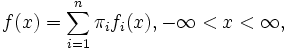
These biological facts do not appear to be controversial. However, they are based on a series of different sexual dimorphism measures, or indices. Sexual dimorphism, in most works, is measured on the assumption that a random variable is being taken into account. This means that there is a law which accounts for the behavior of the whole set of values that compose the domain of the random variable, a law which is called distribution function. Because both studies of sexual dimorphism aim at establishing differences, in some random variable, between sexes and the behavior of the random variable is accounted for by its distribution function, it follows that a sexual dimorphism study should be equivalent to a study whose main purpose is to determine to what extent the two distribution functions - one per sex - overlap (see shaded area in Fig. 1, where two normal distributions are represented).

Measures based on sample means
In Borgognini Tarli and Repetto (1986) an account of indices based on sample means can be seen. Perhaps, the most widely used is the quotient,

where  is the sample mean of one sex (e.g., male) and
  the corresponding mean of the other. Nonetheless, for instance,

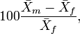
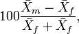
have also been proposed.
Going over the works where these indices are used, the reader misses any reference to their parametric counterpart (see reference above). In other words, if we suppose that the quotient of two sample means is considered, no work can be found where, in order to make inferences, the way in which the quotient is used as a point estimate of

is discussed.
By assuming that differences between populations are the objective to analyze, when quotients of sample means are used it is important to point out that the only feature of these populations that seems to be interesting is the mean parameter. However, a population has also variance, as well as a shape which is defined by its distribution function (notice that, in general, this function depends on parameters such as means or variances).
Measures based on something more than sample means
Marini et al. (1999) have illustrated that it is a good idea to consider something other than sample means when sexual dimorphism is analyzed. Possibly, the main reason is that the intrasexual variability influences both the manifestation of dimorphism and its interpretation.
Normal populations
Sample functions
It is likely that, within this type of indices, the one used the most is the well-known statistic with Student's t distribution (see, for instance, Green, 1989). Marini et al. (1999) have observed that variability among females seems to be lower than among males, so that it appears advisable to use the form of the Student's t statistic with degrees of freedom given by the Welch-Satterthwaite approximation,
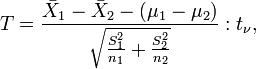
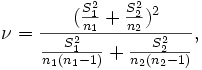
where  are sample variances and sample sizes, respectively.
Anyway, it is important to point out the following,
- when this statistic is taken into account in sexual dimorphism studies, two normal populations are involved. From these populations two random samples are extracted, each one corresponding to a sex, and such samples are independent.
- when inferences are considered, what we are testing by using this statistic is that the difference between two mathematical expectations is a hypothesized value, say
However, in sexual dimorphism analyses, it does not appear reasonably (see Ipiña and Durand, 2000) to assume that two independent random samples have been selected. Rather on the contrary, when we sample we select some random observations - making up one sample - that sometimes correspond to one sex and sometimes to the other.
Taking parameters into account
Chakraborty and Majumder (1982) have proposed an index of sexual dimorphism that is the overlapping area - to be precise, its complement - of two normal density functions (see Fig. 1). Therefore, it is a function of four parameters  (expected values and variances, respectively), and takes the shape of the two normals into account. Inman and Bradley (1989) have discussed this overlapping area as a measure to assess the distance between two normal densities.
Regarding inferences, Chakraborty and Majumder proposed a sample function constructed by considering the Laplace-DeMoivre's theorem (an application to binomial laws of the central limit theorem). According to these authors, the variance of such a statistic is,
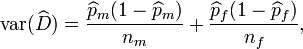
where  is the statistic, and
 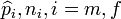 (male, female) stand for the estimate of the probability of observing the measurement of an individual of the
  sex in some interval of the real line, and the sample size of the i sex, respectively. Notice that this implies that two independent random variables with binomial distributions have to be regarded. One of such variables is number of individuals of the f sex in a sample of size
  composed of individuals of the f sex, which seems nonsensical.
Mixture models
Authors such as Josephson et al. (1996) believe that the two sexes to be analyzed form a single population with a probabilistic behavior denominated a mixture of two normal populations. Thus, if  is a random variable which is normally distributed among the females of a population and likewise this variable is normally distributed among the males of the population, then,
is the density of the mixture with two normal components, where  are the normal densities and the mixing proportions of both sexes, respectively. See an example in Fig. 2 where the thicker curve represents the mixture whereas the thinner curves are the
  functions.

It is from a population modelled like this that a random sample with individuals of both sexes can be selected. Note that on this sample tests which are based on the normal assumption cannot be applied since, in a mixture of two normal components, is not a normal density.
Josephson et al. limited themselves to considering two normal mixtures with the same component variances and mixing proportions. As a consequence, their proposal to measure sexual dimorphism is the difference between the mean parameters of the two normals involved. In estimating these central parameters, the procedure used by Josephson et al. is the one of Pearson's moments. Nowadays, the EM expectation maximization algorithm (see McLachlan and Basford, 1988) and the MCMC Markov chain Monte Carlo Bayesian procedure (see Gilks et al., 1996) are the two competitors for estimating mixture parameters.
Possibly the main difference between considering two independent normal populations and a mixture model of two normal components is in the mixing proportions, which is the same as saying that in the two independent normal population model the interaction between sexes is ignored. This, in turn implies that probabilistic properties change (see Ipiña and Durand, 2000).
The MI measure
Ipiña and Durand (2000, 2004) have proposed a measure of sexual dimorphism called  . This proposal computes the overlapping area between the
  and
and  functions, which represent the contribution of each sex to the two normal components mixture (see shaded area in Fig. 2). Thus, can be written,
![MI = \int_R \operatorname{min}[\pi_1f_1(x), (1 - \pi_1)f_2(x)]\,dx ,](../I/m/15d044ce6e75f341beedabcbc6a24328.png)
 being the real line.
The smaller the overlapping area the greater the gap between the two functions and , in which case the sexual dimorphism is greater. Obviously, this index is a function of the five parameters that characterize a mixture of two normal components (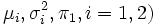 . Its range is in the interval
 ![(0, 0.5]](../I/m/ba3615f9099a19e749d18c97216f351d.png) , and the interested reader can see, in the work of the authors who proposed the index, the way in which an interval estimate is constructed.
, and the interested reader can see, in the work of the authors who proposed the index, the way in which an interval estimate is constructed.
Measures based on non-parametric methods
Marini et al. (1999) have suggested the Kolmogorov-Smirnov distance as a measure of sexual dimorphism. The authors use the following form of the statistic,

with  being sample cumulative distributions corresponding to two independent random samples.
Such a distance has the advantage of being applicable whatever the form of the random variable distributions concerned, yet they should be continuous. The use of this distance assumes that two populations are involved. Further, the Kolmogorov-Smirnov distance is a sample function whose aim is to test that the two samples under analysis have been selected from a single distribution. If one accepts the null hypothesis, then there is not sexual dimorphism; otherwise, there is.
See also
References
- Alexander, R.D., Hoogland, J.L., Howard, R.D., Noonan, K.M. and Sherman, P.W. (1979) Sexual dimorphism and breeding systems in pinnipeds, ungulates, primates and humans, in Evolutionary Biology and Human Social Behavior: An Anthropological Perspective, N.A. Chagnon and W. Irons, Scituate, M.A.: Duxbury Press, 402-435.
- Borgognini Tarli, S.M. and Repetto, E. (1986) Methodological considerations on the study of sexual dimorphism in past human populations. Hum. Evol. 1: 51-56.
- Chakraborty, R. and Majumder, P.P. (1982) On Bennet's measure of sex dimorphism. Am. J. Phys. Anthrop. 59: 295-298.
- Clutton-Brock, T.H. (1985) Size, sexual dimorphism and polygamy in primates, in Size and Scaling in Primate Biology, W.L. Jungers, N. York: Plenum, 211-237.
- Fleagle, J.G., Kay, R.F. and Simons, E.L. (1980) Sexual dimorphism in early anthropoids. Nature 287: 328-330.
- Gilks, W.R., Richardson, S. and Spiegelhalter, D.J. (1996) Markov Chain Monte Carlo in Practice. London: Chapman and Hall.
- Green, D.L. (1989) Comparison of t-tests for differences in sexual dimorphism between populations. Am. J. Phys. Anthropol. 79: 121-125.
- Inman, H.F. and Bradley, E.L. (1989) The overlapping coefficient as a measure of agreement between probability distributions and point estimation of the overlap of two normal densities. Commun. Statist.-Theory Meth. 18: 3851-3874.
- Ipiña, S.L. and Durand, A.I. (2000) A measure of sexual dimorphism in populations which are univariate normal mixtures. Bull. Math. Biol. 62: 925-941.
- Ipiña, S.L. and Durand, A.I. (2004) Inferential assessment of the MI index of sexual dimorphism: A comparative study with some other sexual dimorphism measures. Bull. Math. Biol. 66: 505-522.
- Josephson, S.C., Juell, K.E. and Rogers, A.R. (1996) Estimating sexual dimorphism by method of moments. Am. J. Phys. Anthropol. 100: 191-206.
- Kappelman, J. (1996) The evolution of body mass and relative brain size in fossil hominids. J. Hum. Evol. 30: 243-276.
- Kay, R.F. (1982) Sivapithecus simonsi a new species of Miocene hominoid with comments on the phylogenetic status of Ramapithecinae. Int. J. Primatol. 3: 113-173.
- Kelley, J. (1993) Taxonomic implications of sexual dimorphism in Lufengpithecus, in Species, Species Concepts, and Primate Evolution, W.H. Kimbel and L.B. Martin, N. York: Plenum, 429-458.
- Klein, R.G. and Cruz-Uribe, K. (1983) The Analysis of Animal Bones from Archaeological Sites. Chicago: University of Chicago Press.
- Lovejoy, C.O. (1981) The origin of man. Science 211: 341-350.
- Marini, E. Racugno, W. and Borgognini Tarli, S.M. (1999) Univariate estimates of sexual dimorphism: the effects of intrasexual variability. Am. J. Phys. Anthrop. 109: 501-508.
- McLachlan, G.J. and Basford, K.E. (1988) Mixture Models. Inference and Applications to Clustering. N. York: Marcel Dekker Inc.
- Oxnard, C.E. (1987) Fossils, Teeth and Sex: New Perspective in Human Evolution. Seattle: University of Washington Press.
- Plavcan, J.M. and van Schaick, C.P. (1992) Intrasexual competition and canine dimorphism in anthropoid primates. Am. J. Phys. Anthropol. 87: 461-477.