Sensor array
A sensor array is a group of sensors, usually deployed in a certain geometry pattern, used for collecting and processing electromagnetic or acoustic signals. The advantage of using a sensor array over using a single sensor lies in the fact that an array adds new dimensions to the observation, helping to estimate more parameters and improve the estimation performance. For example an array of radio antenna elements used for beamforming can increase antenna gain in the direction of the signal while decreasing the gain in other directions, i.e., increasing signal-to-noise ratio (SNR) by amplifying the signal coherently. Another example of sensor array application is to estimate the direction of arrival of impinging electromagnetic waves. The related processing method is called array signal processing. Application examples of array signal processing include radar/sonar, wireless communications, seismology, machine condition monitoring, astronomical observations fault diagnosis, etc.
Using array signal processing, the temporal and spatial properties (or parameters) of the impinging signals interfered by noise and hidden in the data collected by the sensor array can be estimated and revealed. This is known as parameter estimation.
Principles
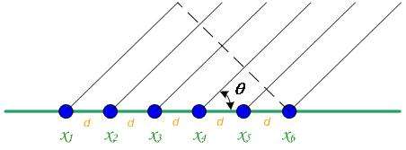
Figure 1 illustrates a six-element uniform linear array (ULA). In this example, the sensor array is assumed to be in the far-field of a signal source so that it can be treated as planar wave.
Parameter estimation takes advantage of the fact that the distance from the source to each antenna in the array is different, which means that the input data at each antenna will be phase-shifted replicas of each other. Eq. (1) shows the calculation for the extra time it takes to reach each antenna in the array relative to the first one, where c is the velocity of light.

Each sensor is associated with a different delay. The delays are small but not trivial. In frequency domain, they are displayed as phase shift among the signals received by the sensors. The delays are closely related to the incident angle and the geometry of the sensor array. Given the geometry of the array, the delays or phase differences can be used to estimate the incident angle. Eq. (1) is the mathematical basis behind array signal processing. Simply summing the signals received by the sensors and calculating the mean value give the result
.

Because the received signals are out of phase, this mean value does not give an enhanced signal compared with the original source. Heuristically, if we can find weights multiplying to the received signals to set them in phase prior to the summation, the mean value
![y={\frac {1}{M}}\sum _{{i=1}}^{{M}}[{\boldsymbol w}_{i}{\boldsymbol x}_{i}(t-\Delta t_{i})]\ \ (3)](../I/m/5d65395aa3f3e783f404d9173d16fb0f0795bc03.svg)
will result in an enhanced signal. The process of multiplying a well selected set of weights to the signals received by the sensor array so that the signal is added constructively while suppressing the noise is called beamforming. There are a variety of beamforming algorithms for sensor arrays, such as the delay-and-sum approach, spectral based (non-parametric) approaches and parametric approaches. These beamforming algorithms are briefly described as follows.
Array design
Sensor arrays have different geometrical designs, including linear, circular, planar, cylindrical and spherical arrays. There are sensor arrays with arbitrary array configuration, which require more complex signal processing techniques for parameter estimation. In uniform linear array (ULA) the phase of the incoming signal should be limited to to avoid grating waves. It means that for angle of arrival in the interval sensor spacing should be smaller than half the wavelength . However, the width of the main beam, i.e., the resolution or directivity of the array, is determined by the length of the array compared to the wavelength. In order to have a decent directional resolution the length of the array should be several times larger than the radio wavelength.


![[-{\frac {\pi }{2}},{\frac {\pi }{2}}]](../I/m/9dc480741da18128936a24486e90845e818ee6ff.svg)

Types of sensor arrays
Antenna array
- Antenna array (electromagnetic), a geometrical arrangement of antenna elements with a deliberate relationship between their currents, forming a single antenna usually to achieve a desired radiation pattern
- Directional array, an antenna array optimized for directionality
- Phased array, An antenna array where the phase shifts (and amplitudes) applied to the elements are modified electronically, typically in order to steer the antenna system's directional pattern, without the use of moving parts
- Smart antenna, a phased array in which a signal processor computes phase shifts to optimize reception and/or transmission to a receiver on the fly, such as is performed by cellular telephone towers
- Interferometric array of radio telescopes or optical telescopes, used to achieve high resolution through interferometric correlation
- Watson-Watt / Adcock antenna array, using the Watson-Watt technique whereby two Adcock antenna pairs are used to perform an amplitude comparison on the incoming signal
Acoustic arrays
- Microphone array is used in acoustic measurement and beamforming
- Loudspeaker array is used in acoustic measurement and beamforming
Other arrays
- Geophone array used in Reflection seismology
- Sonar array is an array of hydrophones used in underwater imaging
Delay-and-sum beamforming
If a time delay is added to the recorded signal from each microphone that is equal and opposite of the delay caused by the additional travel time, it will result in signals that are perfectly in-phase with each other. Summing these in-phase signals will result in constructive interference that will amplify the SNR by the number of antennas in the array. This is known as delay-and-sum beamforming. For direction of arrival (DOA) estimation, one can iteratively test time delays for all possible directions. If the guess is wrong, the signal will be interfered destructively, resulting in a diminished output signal, but the correct guess will result in the signal amplification described above.
The problem is, before the incident angle is estimated, how could it be possible to know the time delay that is 'equal' and opposite of the delay caused by the extra travel time? It is impossible. The solution is to try a series of angles at sufficiently high resolution, and calculate the resulting mean output signal of the array using Eq. (3). The trial angle that maximizes the mean output is an estimation of DOA given by the delay-and-sum beamformer. Adding an opposite delay to the input signals is equivalent to rotating the sensor array physically. Therefore, it is also known as beam steering.
![{\hat {\theta }}\in [0,\pi ]](../I/m/9eff0445cdcff72045a4e48c0cc1941c413e2a2f.svg)
Spectrum-based beamforming
Delay and sum beamforming is a time domain approach. It is simple to implement, but it may poorly estimate direction of arrival (DOA): if the signal is contaminated with strong noise, it might be difficult to implement the algorithm. The solution to this is a frequency domain approach. The Fourier transform transforms the signal from the time domain to the frequency domain. This converts the time delay between adjacent sensors into a phase shift. Thus, the array output vector at any time t can be denoted as , where stands for the signal received by the first sensor. Frequency domain beamforming algorithms use the spatial covariance matrix, represented by . This M by M matrix carries the spatial and spectral information of the incoming signals. Assuming zero-mean Gaussian white noise, the basic model of the spatial covariance matrix is given by


where is the variance of the white noise, is the identity matrix and is the array manifold vector with . This model is of central importance in frequency domain beamforming algorithms.


Some spectrum-based beamforming approaches are listed below.
Conventional (Bartlett) beamformer
The Bartlett beamformer is a natural extension of conventional spectral analysis (spectrogram) to the sensor array. Its spectral power is represented by
.

The angle that maximizes this power is an estimation of the angle of arrival.
MVDR (Capon) beamformer
The Minimum Variance Distortionless Response beamformer, also known as the Capon beamforming algorithm, has a power given by
.

Though the MVDR/Capon beamformer can achieve better resolution than the conventional (Bartlett) approach, but this algorithm has higher complexity due to the full-rank matrix inversion. Technical advances in GPU computing have begun to narrow this gap and make real-time Capon beamforming possible.[1]
MUSIC beamformer
MUSIC (MUltiple SIgnal Classification) beamforming algorithm starts with decomposing the covariance matrix as given by Eq. (4) for both the signal part and the noise part. The eigen-decomposition of is represented by
.

MUSIC uses the noise sub-space of the spatial covariance matrix in the denominator of the Capon algorithm
.

Therefore MUSIC beamformer is also known as subspace beamformer. Compared to the Capon beamformer, it gives much better DOA estimation.
Parametric beamformers
One of the major advantages of the spectrum based beamformers is a lower computational complexity, but they may not give accurate DOA estimation if the signals are correlated or coherent. An alternative approach are parametric beamformers, also known as maximum likelihood (ML) beamformers. One example of a maximum likelihood method commonly used in engineering is the least squares method. In the least square approach, a quadratic penalty function is used. To get the minimum value (or least squared error) of the quadratic penalty function (or objective function), take its derivative (which is linear), let it equal zero and solve a system of linear equations.
In ML beamformers the quadratic penalty function is used to the spatial covariance matrix and the signal model. One example of ML beamformer penalty function is
,

where is the Frobenius norm. It can be seen in Eq. (4) that the penalty function of Eq. (9) is minimized by approximating the signal model to the sample covariance matrix as accurate as possible. In other words, the maximum likelihood beamformer is to find the DOA , the independent variable of matrix , so that the penalty function in Eq. (9) is minimized. In practice, the penalty function may look different, depending on the signal and noise model. For this reason, there are two major categories of maximum likelihood beamformers: Deterministic ML beamformers and stochastic ML beamformers, corresponding to a deterministic and a stochastic model, respectively.

Another idea to change the former penalty equation is the consideration of simplifying the minimization by differentiation of the penalty function. In order to simplify the optimization algorithm, logarithmic operations and the probability density function (PDF) of the observations may be used in some ML beamformers.
The optimizing problem is solved by finding the roots of the derivative of the penalty function after equating it with zero. Because the equation is non-linear a numerical searching approach such as Newton–Raphson method is usually employed. The Newton–Raphson method is an iterative root search method with the iteration
.

The search starts from an initial guess . If the Newton-Raphson search method is employed to minimize the beamforming penalty function, the resulting beamformer is called Newton ML beamformer. Several well-known ML beamformers are described below without providing further details due to the complexity of the expressions.

- Deterministic maximum likelihood meamformer
- In deterministic maximum likelihood meamformer (DML), the noise is modeled as a stationary Gaussian white random processes while the signal waveform as deterministic (but arbitrary) and unknown.
- Stochastic maximum likelihood meamformer
- In stochastic maximum likelihood meamformer (SML), the noise is modeled as stationary Gaussian white random processes (the same as in DML) whereas the signal waveform as Gaussian random processes.
- Method of direction estimation
- Method of direction estimation (MODE) is subspace maximum likelihood beamformer, just as MUSIC, is the subspace spectral based beamformer. Subspace ML beamforming is obtained by eigen-decomposition of the sample covariance matrix.
References
- ↑ Asen, Jon Petter; Buskenes, Jo Inge; Nilsen, Carl-Inge Colombo; Austeng, Andreas; Holm, Sverre (2014). "Implementing capon beamforming on a GPU for real-time cardiac ultrasound imaging". IEEE Transactions on Ultrasonics, Ferroelectrics, and Frequency Control. 61: 76. doi:10.1109/TUFFC.2014.6689777.
Further reading
- H. L. Van Trees, “Optimum array processing – Part IV of detection, estimation, and modulation theory”, John Wiley, 2002
- H. Krim and M. Viberg, “Two decades of array signal processing research”, IEEE Transactions on Signal Processing Magazine, July 1996
- S. Haykin, Ed., “Array Signal Processing”, Eaglewood Cliffs, NJ: Prentice-Hall, 1985
- S. U. Pillai, “Array Signal Processing”, New York: Springer-Verlag, 1989
- P. Stoica and R. Moses, “Introduction to Spectral Analysis", Prentice-Hall, Englewood Cliffs, USA, 1997. available for download.
- J. Li and P. Stoica, “Robust Adaptive Beamforming", John Wiley, 2006.
- J. Cadzow, “Multiple Source Location—The Signal Subspace Approach”, IEEE Transactions on Acoustics, Speech and Signal Processing, Vol. 38, No. 7, July 1990
- G. Bienvenu and L. Kopp, “Optimality of high resolution array processing using the eigensystem approach”, IEEE Transactions on Acoustics, Speech and Signal Process, Vol. ASSP-31, pp. 1234–1248, October 1983
- I. Ziskind and M. Wax, “Maximum likelihood localization of multiple sources by alternating projection”, IEEE Transactions on Acoustics, Speech and Signal Process, Vol. ASSP-36, pp. 1553–1560, October 1988
- B. Ottersten, M. Verberg, P. Stoica, and A. Nehorai, “Exact and large sample maximum likelihood techniques for parameter estimation and detection in array processing”, Radar Array Processing, Springer-Verlag, Berlin, pp. 99–151, 1993
- M. Viberg, B. Ottersten, and T. Kailath, “Detection and estimation in sensor arrays using weighted subspace fitting”, IEEE Transactions on Signal Processing, vol. SP-39, pp 2346–2449, November 1991
- M. Feder and E. Weinstein, “Parameter estimation of superimposed signals using the EM algorithm”, IEEE Transactions on Acoustic, Speech and Signal Proceeding, vol ASSP-36, pp. 447–489, April 1988
- Y. Bresler and Macovski, “Exact maximum likelihood parameter estimation of superimposed exponential signals in noise”, IEEE Transactions on Acoustic, Speech and Signal Proceeding, vol ASSP-34, pp. 1081–1089, October 1986
- R. O. Schmidt, “New mathematical tools in direction finding and spectral analysis”, Proceedings of SPIE 27th Annual Symposium, San Diego, California, August 1983