Seismic tomography
Seismic tomography is a technique for imaging the subsurface of the Earth with seismic waves produced by earthquakes or explosions. P-, S-, and surface waves can be used for tomographic models of different resolutions based on seismic wavelength, wave source distance, and the seismograph array coverage.[1] The data received at seismometers are used to solve an inverse problem, wherein the locations of reflection and refraction of the wave paths are determined. This solution can be used to create 3D images of velocity anomalies which may be interpreted as structural, thermal, or compositional variations. Geoscientists use these images to better understand core, mantle, and plate tectonic processes.
Theory
Tomography is solved as an inverse problem. Seismic travel time data are compared to an initial Earth model and the model is modified until the best possible fit between the model predictions and observed data is found. Seismic waves would travel in straight lines if Earth was of uniform composition, but the compositional layering, tectonic structure, and thermal variations reflect and refract seismic waves. The location and magnitude of these variations can be calculated by the inversion process, although solutions to tomographic inversions are non-unique.
Seismic tomography is similar to medical x-ray computed tomography (CT scan) in that a computer processes receiver data to produce a 3D image, although CT scans use attenuation instead of traveltime difference. Seismic tomography has to deal with the analysis of curved ray paths which are reflected and refracted within the earth and potential uncertainty in the location of the earthquake hypocenter. CT scans use linear x-rays and a known source.[2]
History
Seismic tomography requires large datasets of seismograms and well-located earthquake or explosion sources. These became more widely available in the 1960s with the expansion of global seismic networks and in the 1970s when digital seismograph data archives were established. These developments occurred concurrently with advancements in computing power that were required to solve inverse problems and generate theoretical seismograms for model testing.[3]
In 1977, P-wave delay times were used to create the first seismic array-scale 2D map of seismic velocity.[4] In the same year, P-wave data were used to determine 150 spherical harmonic coefficients for velocity anomalies in the mantle.[1] The first model using iterative techniques, required when there are a large numbers of unknowns, was done in 1984. This built upon the first radially anisotropic model of the Earth, which provided the required initial reference frame to compare tomographic models to for iteration.[5] Initial models had resolution of ~3000 to 5000 km, as compared to the few hundred kilometer resolution of current models.[6]
Seismic tomographic models improve with advancements in computing and expansion of seismic networks. Recent models of global body waves used over 107 traveltimes to model 105 to 106 unknowns.[7]
Process
Seismic tomography uses seismic records to create 2D and 3D images of subsurface anomalies by solving large inverse problems such that generate models consistent with observed data. Various methods are used to resolve anomalies in the crust and lithosphere, shallow mantle, whole mantle, and core based on the availability of data and types of seismic waves that penetrate the region at a suitable wavelength for feature resolution. The accuracy of the model is limited by availability and accuracy of seismic data, wave type utilized, and assumptions made in the model.
P-wave data are used in most local models and global models in areas with sufficient earthquake and seismograph density. S- and surface wave data are used in global models when this coverage is not sufficient, such as in ocean basins and away from subduction zones. First-arrival times are the most widely used, but models utilizing reflected and refracted phases are used in more complex models, such as those imaging the core. Differential traveltimes between wave phases or types are also used.
Local Tomography
Local tomographic models are often based on a temporary seismic array targeting specific areas, unless in a seismically active region with extensive permanent network coverage. These allow for the imaging of the crust and upper mantle.
- Diffraction and wave equation tomography use the full waveform, rather than just the first arrival times. The inversion of amplitude and phases of all arrivals provide more detailed density information than transmission traveltime alone. Despite the theoretical appeal, these methods are not widely employed because of the computing expense and difficult inversions.
- Reflection tomography originated with exploration geophysics. It uses an artificial source to resolve small-scale features at crustal depths. Wide-angle tomography is similar, but with a wide source to receiver offset. This allows for the detection of seismic waves refracted from sub-crustal depths and can determine continental architecture and details of plate margins. These two methods are often used together.
- Local earthquake tomography is used in seismically active regions with sufficient seismometer coverage. Given the proximity between source and receivers, a precise earthquake focus location must be known. This requires the simultaneous iteration of both structure and focus locations in model calculations.[7]
- Teleseismic tomography uses waves from distant earthquakes that deflect upwards to a local seismic array. The models can reach depths similar to the array aperture, typically to depths for imaging the crust and lithosphere (a few hundred kilometers). The waves travel near 30° from vertical, creating a vertical distortion to compact features.[8]
Regional or Global Tomography

Regional to global scale tomographic models are generally based on long wavelengths. Various models have better agreement with each other than local models due to the large feature size they image, such as subducted slabs and superplumes. The trade off from whole mantle to whole earth coverage is the coarse resolution (hundreds of kilometers) and difficulty imaging small features (e.g. narrow plumes). Although often used to image different parts of the subsurface, P- and S-wave derived models broadly agree where there is image overlap. These models use data from both permanent seismic stations and supplementary temporary arrays.
- First arrival traveltime P-wave data are used to generate the highest resolution tomographic images of the mantle. These models are limited to regions with sufficient seismograph coverage and earthquake density, therefore cannot be used for areas such as inactive plate interiors and ocean basins without seismic networks. Other phases of P-waves are used to image the deeper mantle and core.
- In areas with limited seismograph or earthquake coverage, multiple phases of S-waves can be used for tomographic models. These are of lower resolution than P-wave models, due to the distances involved and fewer bounce-phase data available. S-waves can also be used in conjunction with P-waves for differential arrival time models.
- Surface waves can be used for tomography of the crust and upper mantle where no body wave (P and S) data are available. Both Rayleigh and Love waves can be used. The low frequency waves lead to low resolution models, therefore these models have difficulty with crustal structure. Free oscillations, or normal mode seismology, are the long wavelength, low frequency movements of the surface of the earth which can be thought of as a type of surface wave. The frequencies of these oscillations can be obtained through Fourier transformation of seismic data. The models based on this method are of broad scale, but have the advantage of relatively uniform data coverage as compared to data sourced directly from earthquakes.
- Attenuation tomography attempts to extract the anaelastic signal from the elastic-dominated waveform of seismic waves. The advantage of this method is its sensitivity to temperature, thus ability to image thermal features such as mantle plumes and subduction zones. Both surface and body waves have been used in this approach.
- Ambient noise tomography cross-correlates waveforms from random wavefields generated by oceanic and atmospheric disturbances which subsequently become diffuse within the Earth. This method has produced high-resolution images and is an area of active research.
- Waveforms are modeled as rays in seismic analysis, but all waves are affected by the material near the ray path. The finite frequency effect is the result the surrounding medium has on a seismic record. Finite frequency tomography accounts for this in determining both travel time and amplitude anomalies, increasing image resolution. This has the ability to resolve much larger variations (i.e. 10-30%) in material properties.
Applications
Seismic tomography can resolve anisotropy, anelasticity, density, and bulk sound density.[6] Variations in these parameters may be a result of thermal or chemical differences, which are attributed to processes such as mantle plumes, subducting slabs, and mineral phase changes. Larger scale features that can be imaged with tomography include the high velocities beneath continental shields and low velocities under ocean spreading centers.[4]
Hotspots

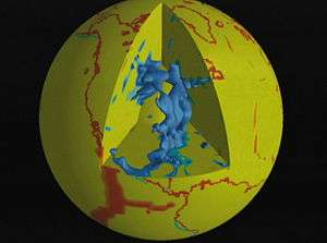
The mantle plume hypothesis proposes that areas of volcanism not readily explained by plate tectonics, called hotspots, are a result of thermal upwelling from as deep as the core-mantle boundary that become diapirs in the crust. This is an actively contested theory,[8] although tomographic images suggest there are anomalies beneath some hotspots. The best imaged of these are large low-shear-velocity provinces, or superplumes, visible on S-wave models of the lower mantle and believed to reflect both thermal and compositional differences.
The Yellowstone hotspot is responsible for volcanism at the Yellowstone Caldera and a series of extinct calderas along the Snake River Plain. The Yellowstone Geodynamic Project sought to image the plume beneath the hotspot.[9] They found a strong low-velocity body from ~30 to 250 km depth beneath Yellowstone and a weaker anomaly from 250 to 650 km depth which dipped 60° west-northwest. The authors attribute these features to the mantle plume beneath the hotspot being deflected eastward by flow in the upper mantle seen in S-wave models.
The Hawaii hotspot lies beneath the Hawaiian Islands and Emperor Seamounts. Tomographic images show it to be 500 to 600 km wide and up to 2,000 km deep.
Subduction zones
Subducting plates are colder than the mantle into which they are moving. This creates a fast anomaly that is visible in tomographic images. Both the Farallon plate that subducted beneath the west coast of North America[10] and the northern portion of the Indian plate that has subducted beneath Asia[11] have been imaged with tomography.
Limitations
Global seismic networks have expanded steadily since the 1960s, but are still concentrated on continents and in seismically active regions. Oceans, particularly in the southern hemisphere, are under-covered.[8] Tomographic models in these areas will improve when more data becomes available. The uneven distribution of earthquakes naturally biases models to better resolution in seismically active regions.
The type of wave used in a model limits the resolution it can achieve. Longer wavelengths are able to penetrate deeper into the earth, but can only be used to resolve large features. Finer resolution can be achieved with surface waves, with the trade off that they cannot be used in models of the deep mantle. The disparity between wavelength and feature scale causes anomalies to appear of reduced magnitude and size in images. P- and S-wave models respond differently to the types of anomalies depending on the driving material property. First arrival time based models naturally prefer faster pathways, causing models based on these data to have lower resolution of slow (often hot) features.[7] Shallow models must also consider the significant lateral velocity variations in continental crust.
Seismic tomography provides only the current velocity anomalies. Any prior structures are unknown and the slow rates of movement in the subsurface (mm to cm per year) prohibit resolution of changes over modern timescales.[12]
Tomographic solutions are non-unique. Although statistical methods can be used to analyze the validity of a model, unresolvable uncertainty remains.[7] This contributes to difficulty comparing the validity of different model results.
Computing power limits the amount of seismic data, number of unknowns, mesh size, and iterations in tomographic models. This is of particular importance in ocean basins, which due to limited network coverage and earthquake density require more complex processing of distant data. Shallow oceanic models also require smaller model mesh size due to the thinner crust.[5]
Tomographic images are typically presented with a color ramp representing the strength of the anomalies. This has the consequence of making equal changes appear of differing magnitude based on visual perceptions of color, such as the change from orange to red being more subtle than blue to yellow. The degree of color saturation can also visually skew interpretations. These factors should be considered when analyzing images.[2]
See also
References
- 1 2 Nolet, G. (1987-01-01). Nolet, Guust, ed. Seismic wave propagation and seismic tomography. Seismology and Exploration Geophysics. Springer Netherlands. pp. 1–23. doi:10.1007/978-94-009-3899-1_1#page-1. ISBN 9789027725837.
- 1 2 "Seismic Tomography—Using earthquakes to image Earth's interior". Incorporated Research Institutions for Seismology (IRIS). Retrieved 18 May 2016.
- ↑ "A Brief History of Seismology" (PDF). United States Geologic Survey (USGS). Retrieved 4 May 2016.
- 1 2 Kearey, Philip; Klepeis, Keith A.; Vine, Frederick J. (2013-05-28). Global Tectonics. John Wiley & Sons. ISBN 1118688082.
- 1 2 Liu, Q.; Gu, Y. J. (2012-09-16). "Seismic imaging: From classical to adjoint tomography". Tectonophysics. 566–567: 31–66. doi:10.1016/j.tecto.2012.07.006.
- 1 2 Romanowicz, Barbara (2003-01-01). "GLOBAL MANTLE TOMOGRAPHY: Progress Status in the Past 10 Years". Annual Review of Earth and Planetary Sciences. 31 (1): 303–328. doi:10.1146/annurev.earth.31.091602.113555.
- 1 2 3 4 Rawlinson, N.; Pozgay, S.; Fishwick, S. (2010-02-01). "Seismic tomography: A window into deep Earth". Physics of the Earth and Planetary Interiors. 178 (3–4): 101–135. doi:10.1016/j.pepi.2009.10.002.
- 1 2 3 Julian, Brian (2006). "Seismology: The Hunt for Plumes" (PDF). mantleplumes.org. Retrieved 3 May 2016.
- ↑ Smith, Robert B.; Jordan, Michael; Steinberger, Bernhard; Puskas, Christine M.; Farrell, Jamie; Waite, Gregory P.; Husen, Stephan; Chang, Wu-Lung; O'Connell, Richard (2009-11-20). "Geodynamics of the Yellowstone hotspot and mantle plume: Seismic and GPS imaging, kinematics, and mantle flow". Journal of Volcanology and Geothermal Research. The Track of the Yellowstone HotspotWhat do Neotectonics, Climate Indicators, Volcanism, and Petrogenesis Reveal about Subsurface Processes?. 188 (1–3): 26–56. doi:10.1016/j.jvolgeores.2009.08.020.
- ↑ "Seismic Tomography" (PDF). earthscope.org. Incorporated Research Institutions for Seismology (IRIS). Retrieved 18 May 2016.
- ↑ Replumaz, Anne; Negredo, Ana M.; Guillot, Stéphane; Villaseñor, Antonio (2010-03-01). "Multiple episodes of continental subduction during India/Asia convergence: Insight from seismic tomography and tectonic reconstruction". Tectonophysics. Convergent plate margin dynamics: New perspectives from structural geology, geophysics and geodynamic modelling. 483 (1–2): 125–134. doi:10.1016/j.tecto.2009.10.007.
- ↑ Dziewonski, Adam. "Global Seismic Tomography: What we really can say and what we make up" (PDF). mantleplumes.org. Retrieved 18 May 2016.
External links
- EarthScope Education and Outreach: Seismic Tomography Background. Incorporated Research Institutions for Seismology (IRIS). Retrieved 17 January 2013.
- Tomography Animation. Incorporated Research Institutions for Seismology (IRIS). Retrieved 17 January 2013.