Second derivative
| Part of a series of articles about | ||||||
| Calculus | ||||||
|---|---|---|---|---|---|---|
|
||||||
|
Specialized |
||||||
In calculus, the second derivative, or the second order derivative, of a function f is the derivative of the derivative of f. Roughly speaking, the second derivative measures how the rate of change of a quantity is itself changing; for example, the second derivative of the position of a vehicle with respect to time is the instantaneous acceleration of the vehicle, or the rate at which the velocity of the vehicle is changing with respect to time. In Leibniz notation:

where the last term is the second derivative expression.
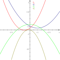
On the graph of a function, the second derivative corresponds to the curvature or concavity of the graph. The graph of a function with a positive second derivative bows downward (that is, is concave when viewed from above), while the graph of a function with a negative second derivative curves in the opposite way.
Second derivative power rule
The power rule for the first derivative, if applied twice, will produce the second derivative power rule as follows:
![{\frac {d^{2}}{dx^{2}}}[x^{n}]={\frac {d}{dx}}{\frac {d}{dx}}[x^{n}]={\frac {d}{dx}}[nx^{n-1}]=n{\frac {d}{dx}}[x^{n-1}]=n(n-1)x^{n-2}.](../I/m/5e1212c1710ab5bb3053aff4ccc15e496bcdab38.svg)
Notation
The second derivative of a function is usually denoted . That is:


When using Leibniz's notation for derivatives, the second derivative of a dependent variable y with respect to an independent variable x is written

This notation is derived from the following formula:

Example
Given the function

the derivative of f is the function

The second derivative of f is the derivative of f′, namely

Relation to the graph


Concavity
The second derivative of a function f measures the concavity of the graph of f. A function whose second derivative is positive will be concave up (sometimes referred to as convex), meaning that the tangent line will lie below the graph of the function. Similarly, a function whose second derivative is negative will be concave down (sometimes called simply “concave”), and its tangent lines will lie above the graph of the function.
Inflection points
If the second derivative of a function changes sign, the graph of the function will switch from concave down to concave up, or vice versa. A point where this occurs is called an inflection point. Assuming the second derivative is continuous, it must take a value of zero at any inflection point, although not every point where the second derivative is zero is necessarily a point of inflection.
Second derivative test
The relation between the second derivative and the graph can be used to test whether a stationary point for a function (i.e. a point where ) is a local maximum or a local minimum. Specifically,

- If then has a local maximum at .
- If then has a local minimum at .
- If , the second derivative test says nothing about the point , a possible inflection point.


The reason the second derivative produces these results can be seen by way of a real-world analogy. Consider a vehicle that at first is moving forward at a great velocity, but with a negative acceleration. Clearly the position of the vehicle at the point where the velocity reaches zero will be the maximum distance from the starting position – after this time, the velocity will become negative and the vehicle will reverse. The same is true for the minimum, with a vehicle that at first has a very negative velocity but positive acceleration.
Limit
It is possible to write a single limit for the second derivative:

The limit is called the second symmetric derivative.[1][2] Note that the second symmetric derivative may exist even when the (usual) second derivative does not.
The expression on the right can be written as a difference quotient of difference quotients:

This limit can be viewed as a continuous version of the second difference for sequences.
Please note that the existence of the above limit does not mean that the function has a second derivative. The limit above just gives a possibility for calculating the second derivative but does not provide a definition. As a counterexample look on the sign function which is defined through


The sign function is not continuous at zero and therefore the second derivative for does not exist. But the above limit exists for :


Quadratic approximation
Just as the first derivative is related to linear approximations, the second derivative is related to the best quadratic approximation for a function f. This is the quadratic function whose first and second derivatives are the same as those of f at a given point. The formula for the best quadratic approximation to a function f around the point x = a is

This quadratic approximation is the second-order Taylor polynomial for the function centered at x = a.
Eigenvalues and eigenvectors of the second derivative
For many combinations of boundary conditions explicit formulas for eigenvalues and eigenvectors of the second derivative can be obtained. For example, assuming and homogeneous Dirichlet boundary conditions, i.e., , the eigenvalues are and the corresponding eigenvectors (also called eigenfunctions) are . Here,
![x\in [0,L]](../I/m/d35e3fa30fa9d0e9f57923fb0101848d4fea625a.svg)


For other well-known cases, see the main article eigenvalues and eigenvectors of the second derivative.
Generalization to higher dimensions
The Hessian
The second derivative generalizes to higher dimensions through the notion of second partial derivatives. For a function f:R3 → R, these include the three second-order partials

and the mixed partials

If the function's image and domain both have a potential, then these fit together into a symmetric matrix known as the Hessian. The eigenvalues of this matrix can be used to implement a multivariable analogue of the second derivative test. (See also the second partial derivative test.)
The Laplacian
Another common generalization of the second derivative is the Laplacian. This is the differential operator defined by


The Laplacian of a function is equal to the divergence of the gradient and the trace of the Hessian matrix.
See also
- Chirpyness, second derivative of instantaneous phase
References
- Anton, Howard; Bivens, Irl; Davis, Stephen (February 2, 2005), Calculus: Early Transcendentals Single and Multivariable (8th ed.), New York: Wiley, ISBN 978-0-471-47244-5
- Apostol, Tom M. (June 1967), Calculus, Vol. 1: One-Variable Calculus with an Introduction to Linear Algebra, 1 (2nd ed.), Wiley, ISBN 978-0-471-00005-1
- Apostol, Tom M. (June 1969), Calculus, Vol. 2: Multi-Variable Calculus and Linear Algebra with Applications, 1 (2nd ed.), Wiley, ISBN 978-0-471-00007-5
- Eves, Howard (January 2, 1990), An Introduction to the History of Mathematics (6th ed.), Brooks Cole, ISBN 978-0-03-029558-4
- Larson, Ron; Hostetler, Robert P.; Edwards, Bruce H. (February 28, 2006), Calculus: Early Transcendental Functions (4th ed.), Houghton Mifflin Company, ISBN 978-0-618-60624-5
- Spivak, Michael (September 1994), Calculus (3rd ed.), Publish or Perish, ISBN 978-0-914098-89-8
- Stewart, James (December 24, 2002), Calculus (5th ed.), Brooks Cole, ISBN 978-0-534-39339-7
- Thompson, Silvanus P. (September 8, 1998), Calculus Made Easy (Revised, Updated, Expanded ed.), New York: St. Martin's Press, ISBN 978-0-312-18548-0
Online books
- Crowell, Benjamin (2003), Calculus
- Garrett, Paul (2004), Notes on First-Year Calculus
- Hussain, Faraz (2006), Understanding Calculus
- Keisler, H. Jerome (2000), Elementary Calculus: An Approach Using Infinitesimals
- Mauch, Sean (2004), Unabridged Version of Sean's Applied Math Book
- Sloughter, Dan (2000), Difference Equations to Differential Equations
- Strang, Gilbert (1991), Calculus
- Stroyan, Keith D. (1997), A Brief Introduction to Infinitesimal Calculus
- Wikibooks, Calculus