Schrödinger equation

For a more general introduction to the topic, see Introduction to quantum mechanics.

Quantum mechanics
${\hat {H}}\|\psi (t)\rangle =i\hbar {\frac {\partial }{\partial t}}\|\psi (t)\rangle$ Schrödinger equation
Introduction Glossary History
Background Classical mechanics Old quantum theory Bra–ket notation Hamiltonian Interference
Fundamentals Complementarity Decoherence Entanglement Energy level Measurement Nonlocality Quantum number State Superposition Symmetry Tunnelling Uncertainty Wave function (collapse)
Experiments Afshar Bell's inequality Davisson–Germer Double-slit Elitzur–Vaidman Franck–Hertz Mach–Zehnder Popper Quantum eraser (delayed-choice) Schrödinger's cat Stern–Gerlach Wheeler's delayed-choice
Formulations Overview Heisenberg Interaction Matrix Phase-space Schrödinger Sum-over-histories (path integral)
Equations Dirac Klein–Gordon Pauli Rydberg Schrödinger
Interpretations Overview Consistent histories Copenhagen de Broglie–Bohm Ensemble Hidden-variable Many-worlds Objective collapse Bayesian Quantum logic Relational Stochastic Scale relativity Transactional
Advanced topics Quantum chaos Quantum computing Density matrix Quantum field theory Fractional quantum mechanics Quantum information science Relativistic quantum mechanics Scattering theory Quantum statistical mechanics
Scientists Aharonov Bell Blackett Bloch Bohm Bohr Born Bose de Broglie Candlin Compton Dirac Davisson Debye Ehrenfest Einstein Everett Fock Fermi Feynman Glauber Gutzwiller Heisenberg Hilbert Jordan Kramers Pauli Lamb Landau Laue Moseley Millikan Onnes Planck Rabi Raman Rydberg Schrödinger Sommerfeld von Neumann Weyl Wien Wigner Zeeman Zeilinger

Schrödinger equation as part of a monument in front of Warsaw University's Centre of New Technologies

In quantum mechanics, the Schrödinger equation is a partial differential equation that describes how the quantum state of a quantum system changes with time. It was formulated in late 1925, and published in 1926, by the Austrian physicist Erwin Schrödinger.^[1]

In classical mechanics, Newton's second law ( $F = m a$ ) is used to make a mathematical prediction as to what path a given system will take following a set of known initial conditions. In quantum mechanics, the analogue of Newton's law is Schrödinger's equation for a quantum system (usually atoms, molecules, and subatomic particles whether free, bound, or localised). It is not a simple algebraic equation, but in general a linear partial differential equation, describing the time-evolution of the system's wave function (also called a "state function").^[2]^:1–2

The concept of a wavefunction is a fundamental postulate of quantum mechanics. Using these postulates, Schrödinger's equation can be derived from the fact that the time-evolution operator must be unitary and must therefore be generated by the exponential of a self-adjoint operator, which is the quantum Hamiltonian. This derivation is explained below.

In the Copenhagen interpretation of quantum mechanics, the wave function is the most complete description that can be given of a physical system. Solutions to Schrödinger's equation describe not only molecular, atomic, and subatomic systems, but also macroscopic systems, possibly even the whole universe.^[3]^:292ff Schrödinger's equation is central to all applications of quantum mechanics including quantum field theory which combines special relativity with quantum mechanics. Theories of quantum gravity, such as string theory also do not modify Schrödinger's equation.

The Schrödinger equation is not the only way to make predictions in quantum mechanics—other formulations can be used, such as Werner Heisenberg's matrix mechanics, and Richard Feynman's path integral formulation.

Equation

Time-dependent equation

The form of the Schrödinger equation depends on the physical situation (see below for special cases). The most general form is the time-dependent Schrödinger equation, which gives a description of a system evolving with time:^[4]^:143

A wave function that satisfies the non-relativistic Schrödinger equation with

V = 0

. In other words, this corresponds to a particle traveling freely through empty space. The real part of the wave function is plotted here.

Time-dependent Schrödinger equation (general)

$i\hbar {\frac {\partial }{\partial t}}\Psi (\mathbf {r} ,t)={\hat {H}}\Psi (\mathbf {r} ,t)$

where $i$ is the imaginary unit, $ħ$ is the Planck constant divided by $2π$ , the symbol $\partial / \partial t$ indicates a partial derivative with respect to time $t$ , $Ψ$ (the Greek letter psi) is the wave function of the quantum system, $r$ and $t$ are the position vector and time respectively, and $Ĥ$ is the Hamiltonian operator (which characterizes the total energy of any given wave function and takes different forms depending on the situation).

Each of these three rows is a wave function which satisfies the time-dependent Schrödinger equation for a harmonic oscillator. Left: The real part (blue) and imaginary part (red) of the wave function. Right: The probability distribution of finding the particle with this wave function at a given position. The top two rows are examples of stationary states, which correspond to standing waves. The bottom row is an example of a state which is not a stationary state. The right column illustrates why stationary states are called "stationary".

The most famous example is the non-relativistic Schrödinger equation for a single particle moving in an electric field (but not a magnetic field; see the Pauli equation):^[5]

Time-dependent Schrödinger equation
(single non-relativistic particle)

$i\hbar {\frac {\partial }{\partial t}}\Psi (\mathbf {r} ,t)=\left[{\frac {-\hbar ^{2}}{2\mu }}\nabla ^{2}+V(\mathbf {r} ,t)\right]\Psi (\mathbf {r} ,t)$

where $μ$ is the particle's "reduced mass", $V$ is its potential energy, $\nabla 2$ is the Laplacian (a differential operator), and $Ψ$ is the wave function (more precisely, in this context, it is called the "position-space wave function"). In plain language, it means "total energy equals kinetic energy plus potential energy", but the terms take unfamiliar forms for reasons explained below.

Given the particular differential operators involved, this is a linear partial differential equation. It is also a diffusion equation, but unlike the heat equation, this one is also a wave equation given the imaginary unit present in the transient term.

The term "Schrödinger equation" can refer to both the general equation (first box above), or the specific nonrelativistic version (second box above and variations thereof). The general equation is indeed quite general, used throughout quantum mechanics, for everything from the Dirac equation to quantum field theory, by plugging in various complicated expressions for the Hamiltonian. The specific nonrelativistic version is a simplified approximation to reality, which is quite accurate in many situations, but very inaccurate in others (see relativistic quantum mechanics and relativistic quantum field theory).

To apply the Schrödinger equation, the Hamiltonian operator is set up for the system, accounting for the kinetic and potential energy of the particles constituting the system, then inserted into the Schrödinger equation. The resulting partial differential equation is solved for the wave function, which contains information about the system.

Time-independent equation

The time-dependent Schrödinger equation described above predicts that wave functions can form standing waves, called stationary states (also called "orbitals", as in atomic orbitals or molecular orbitals). These states are important in their own right, and if the stationary states are classified and understood, then it becomes easier to solve the time-dependent Schrödinger equation for any state. Stationary states can also be described by a simpler form of the Schrödinger equation, the time-independent Schrödinger equation. (This is only used when the Hamiltonian itself is not dependent on time explicitly. However, even in this case the total wave function still has a time dependency.)

Time-independent Schrödinger equation (general)

$\operatorname {\hat {H}} \Psi =E\Psi$

In words, the equation states:

When the Hamiltonian operator acts on a certain wave function $Ψ$ , and the result is proportional to the same wave function $Ψ$ , then $Ψ$ is a stationary state, and the proportionality constant, $E$ , is the energy of the state $Ψ$ .

The time-independent Schrödinger equation is discussed further below. In linear algebra terminology, this equation is an eigenvalue equation.

As before, the most famous manifestation is the non-relativistic Schrödinger equation for a single particle moving in an electric field (but not a magnetic field):

Time-independent Schrödinger equation (single non-relativistic particle)

$\left[{\frac {-\hbar ^{2}}{2\mu }}\nabla ^{2}+V(\mathbf {r} )\right]\Psi (\mathbf {r} )=E\Psi (\mathbf {r} )$

with definitions as above.

Derivation

In the modern understanding of quantum mechanics, Schrödinger's equation may be derived as follows.^[6] If the wave-function at time t is given by $\Psi (t)$ , then by the linearity of quantum mechanics the wave-function at time t' must be given by $\Psi (t')=U(t',t)\Psi (t)$ , where $U(t',t)$ is a linear operator. Since time-evolution must preserve the norm of the wave-function, it follows that $U(t',t)$ must be a member of the unitary group of operators acting on wave-functions. We also know that when $t' = t$ , we must have $U(t,t)=1$ . Therefore, expanding the operator $U(t',t)$ for t' close to t, we can write $U(t',t)=1-iH(t'-t)$ where H is a Hermitian operator. This follows from the fact that the Lie algebra corresponding to the unitary group comprises Hermitian operators. Taking the limit as the time-difference $t'-t$ becomes very small, we obtain Schrödinger's equation.

So far, H is only an abstract Hermitian operator. However using the correspondence principle it is possible to show that, in the classical limit, the expectation value of H is indeed the classical energy. The correspondence principle does not completely fix the form of the quantum Hamiltonian due to the uncertainty principle and therefore the precise form of the quantum Hamiltonian must be fixed empirically.

Implications

The Schrödinger equation and its solutions introduced a breakthrough in thinking about physics. Schrödinger's equation was the first of its type, and solutions led to consequences that were very unusual and unexpected for the time.

Total, kinetic, and potential energy

The overall form of the equation is not unusual or unexpected, as it uses the principle of the conservation of energy. The terms of the nonrelativistic Schrödinger equation can be interpreted as total energy of the system, equal to the system kinetic energy plus the system potential energy. In this respect, it is just the same as in classical physics.

Quantization

The Schrödinger equation predicts that if certain properties of a system are measured, the result may be quantized, meaning that only specific discrete values can occur. One example is energy quantization: the energy of an electron in an atom is always one of the quantized energy levels, a fact discovered via atomic spectroscopy. (Energy quantization is discussed below.) Another example is quantization of angular momentum. This was an assumption in the earlier Bohr model of the atom, but it is a prediction of the Schrödinger equation.

Another result of the Schrödinger equation is that not every measurement gives a quantized result in quantum mechanics. For example, position, momentum, time, and (in some situations) energy can have any value across a continuous range.^[7]^:165–167

Measurement and uncertainty

Main articles: Measurement in quantum mechanics, Heisenberg uncertainty principle, and Interpretations of quantum mechanics

In classical mechanics, a particle has, at every moment, an exact position and an exact momentum. These values change deterministically as the particle moves according to Newton's laws. Under the Copenhagen interpretation of quantum mechanics, particles do not have exactly determined properties, and when they are measured, the result is randomly drawn from a probability distribution. The Schrödinger equation predicts what the probability distributions are, but fundamentally cannot predict the exact result of each measurement.

The Heisenberg uncertainty principle is the statement of the inherent measurement uncertainty in quantum mechanics. It states that the more precisely a particle's position is known, the less precisely its momentum is known, and vice versa.

The Schrödinger equation describes the (deterministic) evolution of the wave function of a particle. However, even if the wave function is known exactly, the result of a specific measurement on the wave function is uncertain.

Quantum tunneling

Main article: Quantum tunneling

Quantum tunneling through a barrier. A particle coming from the left does not have enough energy to climb the barrier. However, it can sometimes "tunnel" to the other side.

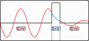
In classical physics, when a ball is rolled slowly up a large hill, it will come to a stop and roll back, because it doesn't have enough energy to get over the top of the hill to the other side. However, the Schrödinger equation predicts that there is a small probability that the ball will get to the other side of the hill, even if it has too little energy to reach the top. This is called quantum tunneling. It is related to the distribution of energy: although the ball's assumed position seems to be on one side of the hill, there is a chance of finding it on the other side.

Particles as waves

Main articles: Matter wave, Wave–particle duality, and Double-slit experiment

A double slit experiment showing the accumulation of electrons on a screen as time passes.

The nonrelativistic Schrödinger equation is a type of partial differential equation called a wave equation. Therefore, it is often said particles can exhibit behavior usually attributed to waves. In some modern interpretations this description is reversed – the quantum state, i.e. wave, is the only genuine physical reality, and under the appropriate conditions it can show features of particle-like behavior. However, Ballentine^[8]^{:Chapter 4, p.99} shows that such an interpretation has problems. Ballentine points out that whilst it is arguable to associate a physical wave with a single particle, there is still only one Schrödinger wave equation for many particles. He points out:

"If a physical wave field were associated with a particle, or if a particle were identified with a wave packet, then corresponding to N interacting particles there should be N interacting waves in ordinary three-dimensional space. But according to (4.6) that is not the case; instead there is one "wave" function in an abstract 3N-dimensional configuration space. The misinterpretation of psi as a physical wave in ordinary space is possible only because the most common applications of quantum mechanics are to one-particle states, for which configuration space and ordinary space are isomorphic."

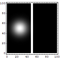
Two-slit diffraction is a famous example of the strange behaviors that waves regularly display, that are not intuitively associated with particles. The overlapping waves from the two slits cancel each other out in some locations, and reinforce each other in other locations, causing a complex pattern to emerge. Intuitively, one would not expect this pattern from firing a single particle at the slits, because the particle should pass through one slit or the other, not a complex overlap of both.

However, since the Schrödinger equation is a wave equation, a single particle fired through a double-slit does show this same pattern (figure on right). Note: The experiment must be repeated many times for the complex pattern to emerge. Although this is counterintuitive, the prediction is correct; in particular, electron diffraction and neutron diffraction are well understood and widely used in science and engineering.

Related to diffraction, particles also display superposition and interference.

The superposition property allows the particle to be in a quantum superposition of two or more quantum states at the same time. However, it is noted that a "quantum state" in QM means the probability that a system will be, for example at a position $x$ , not that the system will actually be at position $x$ . It does not imply that the particle itself may be in two classical states at once. Indeed, QM is generally unable to assign values for properties prior to measurement at all.

Multiverse

In Dublin in 1952 Erwin Schrödinger gave a lecture in which at one point he jocularly warned his audience that what he was about to say might "seem lunatic". It was that, when his Nobel equations seem to be describing several different histories, they are "not alternatives but all really happen simultaneously". This is the earliest known reference to the multiverse.^[9]

Interpretation of the wave function

Main article: Interpretations of quantum mechanics

The Schrödinger equation provides a way to calculate the wave function of a system and how it changes dynamically in time. However, the Schrödinger equation does not directly say what, exactly, the wave function is. Interpretations of quantum mechanics address questions such as what the relation is between the wave function, the underlying reality, and the results of experimental measurements.

An important aspect is the relationship between the Schrödinger equation and wavefunction collapse. In the oldest Copenhagen interpretation, particles follow the Schrödinger equation except during wavefunction collapse, during which they behave entirely differently. The advent of quantum decoherence theory allowed alternative approaches (such as the Everett many-worlds interpretation and consistent histories), wherein the Schrödinger equation is always satisfied, and wavefunction collapse should be explained as a consequence of the Schrödinger equation.

Historical background and development

Erwin Schrödinger

Main article: Theoretical and experimental justification for the Schrödinger equation

Following Max Planck's quantization of light (see black body radiation), Albert Einstein interpreted Planck's quanta to be photons, particles of light, and proposed that the energy of a photon is proportional to its frequency, one of the first signs of wave–particle duality. Since energy and momentum are related in the same way as frequency and wavenumber in special relativity, it followed that the momentum $p$ of a photon is inversely proportional to its wavelength $λ$ , or proportional to its wavenumber $k$ .

p={\frac {h}{\lambda }}=\hbar k

where $h$ is Planck's constant. Louis de Broglie hypothesized that this is true for all particles, even particles which have mass such as electrons. He showed that, assuming that the matter waves propagate along with their particle counterparts, electrons form standing waves, meaning that only certain discrete rotational frequencies about the nucleus of an atom are allowed.^[10] These quantized orbits correspond to discrete energy levels, and de Broglie reproduced the Bohr model formula for the energy levels. The Bohr model was based on the assumed quantization of angular momentum $L$ according to:

L=n{h \over 2\pi }=n\hbar .

According to de Broglie the electron is described by a wave and a whole number of wavelengths must fit along the circumference of the electron's orbit:

n\lambda =2\pi r.\,

This approach essentially confined the electron wave in one dimension, along a circular orbit of radius $r$ .

In 1921, prior to de Broglie, Arthur C. Lunn at the University of Chicago had used the same argument based on the completion of the relativistic energy–momentum 4-vector to derive what we now call the de Broglie relation.^[11] Unlike de Broglie, Lunn went on to formulate the differential equation now known as the Schrödinger equation, and solve for its energy eigenvalues for the hydrogen atom. Unfortunately the paper was rejected by the Physical Review, as recounted by Kamen.^[12]

Following up on de Broglie's ideas, physicist Peter Debye made an offhand comment that if particles behaved as waves, they should satisfy some sort of wave equation. Inspired by Debye's remark, Schrödinger decided to find a proper 3-dimensional wave equation for the electron. He was guided by William R. Hamilton's analogy between mechanics and optics, encoded in the observation that the zero-wavelength limit of optics resembles a mechanical system—the trajectories of light rays become sharp tracks that obey Fermat's principle, an analog of the principle of least action.^[13] A modern version of his reasoning is reproduced below. The equation he found is:^[14]

i\hbar {\frac {\partial }{\partial t}}\Psi (\mathbf {r} ,\,t)=-{\frac {\hbar ^{2}}{2m}}\nabla ^{2}\Psi (\mathbf {r} ,\,t)+V(\mathbf {r} )\Psi (\mathbf {r} ,\,t).

However, by that time, Arnold Sommerfeld had refined the Bohr model with relativistic corrections.^[15]^[16] Schrödinger used the relativistic energy momentum relation to find what is now known as the Klein–Gordon equation in a Coulomb potential (in natural units):

\left(E+{e^{2} \over r}\right)^{2}\psi (x)=-\nabla ^{2}\psi (x)+m^{2}\psi (x).

He found the standing waves of this relativistic equation, but the relativistic corrections disagreed with Sommerfeld's formula. Discouraged, he put away his calculations and secluded himself in an isolated mountain cabin in December 1925.^[17] While at the cabin, Schrödinger decided that his earlier non-relativistic calculations were novel enough to publish, and decided to leave off the problem of relativistic corrections for the future. Despite the difficulties in solving the differential equation for hydrogen (he had sought help from his friend the mathematician Hermann Weyl^[18]^:3) Schrödinger showed that his non-relativistic version of the wave equation produced the correct spectral energies of hydrogen in a paper published in 1926.^[18]^:1^[19] In the equation, Schrödinger computed the hydrogen spectral series by treating a hydrogen atom's electron as a wave

Ψ (x, t)

, moving in a potential well

V

, created by the proton. This computation accurately reproduced the energy levels of the Bohr model. In a paper, Schrödinger himself explained this equation as follows:

“	The already ... mentioned psi-function.... is now the means for predicting probability of measurement results. In it is embodied the momentarily attained sum of theoretically based future expectation, somewhat as laid down in a catalog.	”
	— Erwin Schrödinger^[20]

This 1926 paper was enthusiastically endorsed by Einstein, who saw the matter-waves as an intuitive depiction of nature, as opposed to Heisenberg's matrix mechanics, which he considered overly formal.^[21] The Schrödinger equation details the behavior of

Ψ

but says nothing of its nature. Schrödinger tried to interpret it as a charge density in his fourth paper, but he was unsuccessful.^[22]^:219 In 1926, just a few days after Schrödinger's fourth and final paper was published, Max Born successfully interpreted

Ψ

as the probability amplitude, whose absolute square is equal to probability density.^[22]^:220 Schrödinger, though, always opposed a statistical or probabilistic approach, with its associated discontinuities—much like Einstein, who believed that quantum mechanics was a statistical approximation to an underlying deterministic theory—and never reconciled with the Copenhagen interpretation.^[23] Louis de Broglie in his later years proposed a real valued wave function connected to the complex wave function by a proportionality constant and developed the De Broglie–Bohm theory.

The wave equation for particles

Main article: Wave–particle duality

The Schrödinger equation is a diffusion equation,^[24] the solutions are functions which describe wave-like motions. Wave equations in physics can normally be derived from other physical laws – the wave equation for mechanical vibrations on strings and in matter can be derived from Newton's laws – where the wave function represents the displacement of matter, and electromagnetic waves from Maxwell's equations, where the wave functions are electric and magnetic fields. The basis for Schrödinger's equation, on the other hand, is the energy of the system and a separate postulate of quantum mechanics: the wave function is a description of the system.^[25] The Schrödinger equation is therefore a new concept in itself; as Feynman put it:

“	Where did we get that (equation) from? Nowhere. It is not possible to derive it from anything you know. It came out of the mind of Schrödinger.	”
	— Richard Feynman^[26]

The foundation of the equation is structured to be a linear differential equation based on classical energy conservation, and consistent with the De Broglie relations. The solution is the wave function

ψ

, which contains all the information that can be known about the system. In the Copenhagen interpretation, the modulus of

ψ

is related to the probability the particles are in some spatial configuration at some instant of time. Solving the equation for

ψ

can be used to predict how the particles will behave under the influence of the specified potential and with each other. The Schrödinger equation was developed principally from the De Broglie hypothesis, a wave equation that would describe particles,^[27] and can be constructed as shown informally in the following sections.^[28] For a more rigorous description of Schrödinger's equation, see also Resnick et al.^[29]

Consistency with energy conservation

The total energy

E

of a particle is the sum of kinetic energy

T

and potential energy

V

, this sum is also the frequent expression for the Hamiltonian

H

in classical mechanics:

E=T+V=H\,\!

Explicitly, for a particle in one dimension with position

x

, mass

m

and momentum

p

, and potential energy

V

which generally varies with position and time

t

E={\frac {p^{2}}{2m}}+V(x,t)=H.

For three dimensions, the position vector

r

and momentum vector

p

must be used:

E={\frac {\mathbf {p} \cdot \mathbf {p} }{2m}}+V(\mathbf {r} ,t)=H

This formalism can be extended to any fixed number of particles: the total energy of the system is then the total kinetic energies of the particles, plus the total potential energy, again the Hamiltonian. However, there can be interactions between the particles (an

N

-body problem), so the potential energy

V

can change as the spatial configuration of particles changes, and possibly with time. The potential energy, in general, is not the sum of the separate potential energies for each particle, it is a function of all the spatial positions of the particles. Explicitly:

E=\sum _{n=1}^{N}{\frac {\mathbf {p} _{n}\cdot \mathbf {p} _{n}}{2m_{n}}}+V(\mathbf {r} _{1},\mathbf {r} _{2}\cdots \mathbf {r} _{N},t)=H\,\!

Linearity

The simplest wavefunction is a plane wave of the form:

\Psi (\mathbf {r} ,t)=Ae^{i(\mathbf {k} \cdot \mathbf {r} -\omega t)}\,\!

where the

A

is the amplitude,

k

the wavevector, and

ω

the angular frequency, of the plane wave. In general, physical situations are not purely described by plane waves, so for generality the superposition principle is required; any wave can be made by superposition of sinusoidal plane waves. So if the equation is linear, a linear combination of plane waves is also an allowed solution. Hence a necessary and separate requirement is that the Schrödinger equation is a linear differential equation. For discrete

k

the sum is a superposition of plane waves:

\Psi (\mathbf {r} ,t)=\sum _{n=1}^{\infty }A_{n}e^{i(\mathbf {k} _{n}\cdot \mathbf {r} -\omega _{n}t)}\,\!

for some real amplitude coefficients

A n

, and for continuous

k

the sum becomes an integral, the Fourier transform of a momentum space wavefunction:^[30]

\Psi (\mathbf {r} ,t)={\frac {1}{({\sqrt {2\pi }})^{3}}}\int \Phi (\mathbf {k} )e^{i(\mathbf {k} \cdot \mathbf {r} -\omega t)}d^{3}\mathbf {k} \,\!

where

d 3 k = dk x dk y dk z

is the differential volume element in

k

-space, and the integrals are taken over all

k

-space. The momentum wavefunction

Φ (k)

arises in the integrand since the position and momentum space wavefunctions are Fourier transforms of each other.

Consistency with the De Broglie relations

Diagrammatic summary of the quantities related to the wavefunction, as used in De broglie's hypothesis and development of the Schrödinger equation.^[27]

Einstein's light quanta hypothesis (1905) states that the energy

E

of a photon is proportional to the frequency

ν

(or angular frequency,

ω = 2 π ν

) of the corresponding quantum wavepacket of light:

E=h\nu =\hbar \omega \,\!

Likewise De Broglie's hypothesis (1924) states that any particle can be associated with a wave, and that the momentum

p

of the particle is inversely proportional to the wavelength

λ

of such a wave (or proportional to the wavenumber,

k = 2π / λ

), in one dimension, by:

p={\frac {h}{\lambda }}=\hbar k\;,

while in three dimensions, wavelength

λ

is related to the magnitude of the wavevector

k

\mathbf {p} =\hbar \mathbf {k} \,,\quad |\mathbf {k} |={\frac {2\pi }{\lambda }}\,.

The Planck–Einstein and de Broglie relations illuminate the deep connections between energy with time, and space with momentum, and express wave–particle duality. In practice, natural units comprising

ħ = 1

are used, as the De Broglie equations reduce to identities: allowing momentum, wavenumber, energy and frequency to be used interchangeably, to prevent duplication of quantities, and reduce the number of dimensions of related quantities. For familiarity SI units are still used in this article. Schrödinger's insight, late in 1925, was to express the phase of a plane wave as a complex phase factor using these relations:

\Psi =Ae^{i(\mathbf {k} \cdot \mathbf {r} -\omega t)}=Ae^{i(\mathbf {p} \cdot \mathbf {r} -Et)/\hbar }

and to realize that the first order partial derivatives were: with respect to space:

\nabla \Psi ={\dfrac {i}{\hbar }}\mathbf {p} Ae^{i(\mathbf {p} \cdot \mathbf {r} -Et)/\hbar }={\dfrac {i}{\hbar }}\mathbf {p} \Psi

with respect to time:

{\dfrac {\partial \Psi }{\partial t}}=-{\dfrac {iE}{\hbar }}Ae^{i(\mathbf {p} \cdot \mathbf {r} -Et)/\hbar }=-{\dfrac {iE}{\hbar }}\Psi

Another postulate of quantum mechanics is that all observables are represented by linear Hermitian operators which act on the wavefunction, and the eigenvalues of the operator are the values the observable takes. The previous derivatives are consistent with the energy operator, corresponding to the time derivative,

{\hat {E}}\Psi =i\hbar {\dfrac {\partial }{\partial t}}\Psi =E\Psi

where

E

are the energy eigenvalues, and the momentum operator, corresponding to the spatial derivatives (the gradient

\nabla

{\hat {\mathbf {p} }}\Psi =-i\hbar \nabla \Psi =\mathbf {p} \Psi

where

p

is a vector of the momentum eigenvalues. In the above, the "hats" (

ˆ

) indicate these observables are operators, not simply ordinary numbers or vectors. The energy and momentum operators are differential operators, while the potential energy function

V

is just a multiplicative factor. Substituting the energy and momentum operators into the classical energy conservation equation obtains the operator:

E={\dfrac {\mathbf {p} \cdot \mathbf {p} }{2m}}+V\quad \rightarrow \quad {\hat {E}}={\dfrac {{\hat {\mathbf {p} }}\cdot {\hat {\mathbf {p} }}}{2m}}+V

so in terms of derivatives with respect to time and space, acting this operator on the wavefunction

Ψ

immediately led Schrödinger to his equation:

i\hbar {\dfrac {\partial \Psi }{\partial t}}=-{\dfrac {\hbar ^{2}}{2m}}\nabla ^{2}\Psi +V\Psi

Wave–particle duality can be assessed from these equations as follows. The kinetic energy

T

is related to the square of momentum

p

. As the particle's momentum increases, the kinetic energy increases more rapidly, but since the wavenumber

| k |

increases the wavelength

λ

decreases. In terms of ordinary scalar and vector quantities (not operators):

\mathbf {p} \cdot \mathbf {p} \propto \mathbf {k} \cdot \mathbf {k} \propto T\propto {\dfrac {1}{\lambda ^{2}}}

The kinetic energy is also proportional to the second spatial derivatives, so it is also proportional to the magnitude of the curvature of the wave, in terms of operators:

{\hat {T}}\Psi ={\frac {-\hbar ^{2}}{2m}}\nabla \cdot \nabla \Psi \,\propto \,\nabla ^{2}\Psi \,.

As the curvature increases, the amplitude of the wave alternates between positive and negative more rapidly, and also shortens the wavelength. So the inverse relation between momentum and wavelength is consistent with the energy the particle has, and so the energy of the particle has a connection to a wave, all in the same mathematical formulation.^[27]

Wave and particle motion

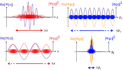
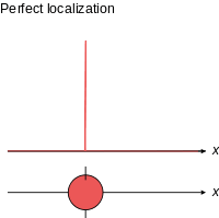
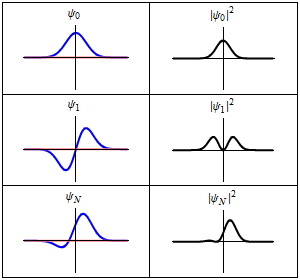
Increasing levels of wavepacket localization, meaning the particle has a more localized position.

In the limit ħ → 0, the particle's position and momentum become known exactly. This is equivalent to the classical particle.

Schrödinger required that a wave packet solution near position

r

with wavevector near

k

will move along the trajectory determined by classical mechanics for times short enough for the spread in

k

(and hence in velocity) not to substantially increase the spread in

r

. Since, for a given spread in

k

, the spread in velocity is proportional to Planck's constant

ħ

, it is sometimes said that in the limit as

ħ

approaches zero, the equations of classical mechanics are restored from quantum mechanics.^[31] Great care is required in how that limit is taken, and in what cases. The limiting short-wavelength is equivalent to

ħ

tending to zero because this is limiting case of increasing the wave packet localization to the definite position of the particle (see images right). Using the Heisenberg uncertainty principle for position and momentum, the products of uncertainty in position and momentum become zero as

ħ \to 0

\sigma (x)\sigma (p_{x})\geqslant {\frac {\hbar }{2}}\quad \rightarrow \quad \sigma (x)\sigma (p_{x})\geqslant 0\,\!

where

σ

denotes the (root mean square) measurement uncertainty in

x

and

p x

(and similarly for the

y

and

z

directions) which implies the position and momentum can only be known to arbitrary precision in this limit. The Schrödinger equation in its general form

i\hbar {\frac {\partial }{\partial t}}\Psi \left(\mathbf {r} ,t\right)={\hat {H}}\Psi \left(\mathbf {r} ,t\right)\,\!

is closely related to the Hamilton–Jacobi equation (HJE)

{\frac {\partial }{\partial t}}S(q_{i},t)=H\left(q_{i},{\frac {\partial S}{\partial q_{i}}},t\right)\,\!

where

S

is action and

H

is the Hamiltonian function (not operator). Here the generalized coordinates

q i

for

i = 1, 2, 3

(used in the context of the HJE) can be set to the position in Cartesian coordinates as

r = (q 1, q 2, q 3) = (x, y, z)

.^[31] Substituting

\Psi ={\sqrt {\rho (\mathbf {r} ,t)}}e^{iS(\mathbf {r} ,t)/\hbar }\,\!

where

ρ

is the probability density, into the Schrödinger equation and then taking the limit

ħ \to 0

in the resulting equation, yields the Hamilton–Jacobi equation. The implications are:

The motion of a particle, described by a (short-wavelength) wave packet solution to the Schrödinger equation, is also described by the Hamilton–Jacobi equation of motion.
The Schrödinger equation includes the wavefunction, so its wave packet solution implies the position of a (quantum) particle is fuzzily spread out in wave fronts. On the contrary, the Hamilton–Jacobi equation applies to a (classical) particle of definite position and momentum, instead the position and momentum at all times (the trajectory) are deterministic and can be simultaneously known.

Non-relativistic quantum mechanics

The quantum mechanics of particles without accounting for the effects of special relativity, for example particles propagating at speeds much less than light, is known as non-relativistic quantum mechanics. Following are several forms of Schrödinger's equation in this context for different situations: time independence and dependence, one and three spatial dimensions, and one and

N

particles. In actuality, the particles constituting the system do not have the numerical labels used in theory. The language of mathematics forces us to label the positions of particles one way or another, otherwise there would be confusion between symbols representing which variables are for which particle.^[29]

Time independent

If the Hamiltonian is not an explicit function of time, the equation is separable into a product of spatial and temporal parts. In general, the wavefunction takes the form:

\Psi ({\text{space coords}},t)=\psi ({\text{space coords}})\tau (t)\,.

where

ψ (space coords)

is a function of all the spatial coordinate(s) of the particle(s) constituting the system only, and

τ (t)

is a function of time only. Substituting for

ψ

into the Schrödinger equation for the relevant number of particles in the relevant number of dimensions, solving by separation of variables implies the general solution of the time-dependent equation has the form:^[14]

\Psi ({\text{space coords}},t)=\psi ({\text{space coords}})e^{-i{Et/\hbar }}\,.

Since the time dependent phase factor is always the same, only the spatial part needs to be solved for in time independent problems. Additionally, the energy operator

Ê = iħ \partial / \partial t

can always be replaced by the energy eigenvalue

E

, thus the time independent Schrödinger equation is an eigenvalue equation for the Hamiltonian operator:^[4]^:143ff

{\hat {H}}\psi =E\psi

This is true for any number of particles in any number of dimensions (in a time independent potential). This case describes the standing wave solutions of the time-dependent equation, which are the states with definite energy (instead of a probability distribution of different energies). In physics, these standing waves are called "stationary states" or "energy eigenstates"; in chemistry they are called "atomic orbitals" or "molecular orbitals". Superpositions of energy eigenstates change their properties according to the relative phases between the energy levels. The energy eigenvalues from this equation form a discrete spectrum of values, so mathematically energy must be quantized. More specifically, the energy eigenstates form a basis – any wavefunction may be written as a sum over the discrete energy states or an integral over continuous energy states, or more generally as an integral over a measure. This is the spectral theorem in mathematics, and in a finite state space it is just a statement of the completeness of the eigenvectors of a Hermitian matrix.

One-dimensional examples

For a particle in one dimension, the Hamiltonian is:

{\hat {H}}={\frac {{\hat {p}}^{2}}{2m}}+V(x)\,,\quad {\hat {p}}=-i\hbar {\frac {d}{dx}}

and substituting this into the general Schrödinger equation gives:

-{\frac {\hbar ^{2}}{2m}}{\frac {d^{2}}{dx^{2}}}\psi (x)+V(x)\psi (x)=E\psi (x)

This is the only case the Schrödinger equation is an ordinary differential equation, rather than a partial differential equation. The general solutions are always of the form:

\Psi (x,t)=\psi (x)e^{-iEt/\hbar }\,.

For

N

particles in one dimension, the Hamiltonian is:

{\hat {H}}=\sum _{n=1}^{N}{\frac {{\hat {p}}_{n}^{2}}{2m_{n}}}+V(x_{1},x_{2},\cdots x_{N})\,,\quad {\hat {p}}_{n}=-i\hbar {\frac {\partial }{\partial x_{n}}}

where the position of particle

n

x n

. The corresponding Schrödinger equation is:

-{\frac {\hbar ^{2}}{2}}\sum _{n=1}^{N}{\frac {1}{m_{n}}}{\frac {\partial ^{2}}{\partial x_{n}^{2}}}\psi (x_{1},x_{2},\cdots x_{N})+V(x_{1},x_{2},\cdots x_{N})\psi (x_{1},x_{2},\cdots x_{N})=E\psi (x_{1},x_{2},\cdots x_{N})\,.

so the general solutions have the form:

\Psi (x_{1},x_{2},\cdots x_{N},t)=e^{-iEt/\hbar }\psi (x_{1},x_{2}\cdots x_{N})

For non-interacting distinguishable particles,^[32] the potential of the system only influences each particle separately, so the total potential energy is the sum of potential energies for each particle:

V(x_{1},x_{2},\cdots x_{N})=\sum _{n=1}^{N}V(x_{n})\,.

and the wavefunction can be written as a product of the wavefunctions for each particle:

\Psi (x_{1},x_{2},\cdots x_{N},t)=e^{-i{Et/\hbar }}\prod _{n=1}^{N}\psi (x_{n})\,,

For non-interacting identical particles, the potential is still a sum, but wavefunction is a bit more complicated – it is a sum over the permutations of products of the separate wavefunctions to account for particle exchange. In general for interacting particles, the above decompositions are not possible.

Free particle

For no potential,

V = 0

, so the particle is free and the equation reads:^[4]^:151ff

-E\psi ={\frac {\hbar ^{2}}{2m}}{d^{2}\psi \over dx^{2}}\,

which has oscillatory solutions for

E > 0

(the

C n

are arbitrary constants):

\psi _{E}(x)=C_{1}e^{i{\sqrt {2mE/\hbar ^{2}}}\,x}+C_{2}e^{-i{\sqrt {2mE/\hbar ^{2}}}\,x}\,

and exponential solutions for

E < 0

\psi _{-|E|}(x)=C_{1}e^{{\sqrt {2m|E|/\hbar ^{2}}}\,x}+C_{2}e^{-{\sqrt {2m|E|/\hbar ^{2}}}\,x}.\,

The exponentially growing solutions have an infinite norm, and are not physical. They are not allowed in a finite volume with periodic or fixed boundary conditions. See also free particle and wavepacket for more discussion on the free particle.

Constant potential

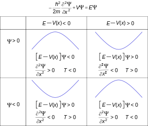
For a constant potential,

V = V 0

, the solution is oscillatory for

E > V 0

and exponential for

E < V 0

, corresponding to energies that are allowed or disallowed in classical mechanics. Oscillatory solutions have a classically allowed energy and correspond to actual classical motions, while the exponential solutions have a disallowed energy and describe a small amount of quantum bleeding into the classically disallowed region, due to quantum tunneling. If the potential

V 0

grows to infinity, the motion is classically confined to a finite region. Viewed far enough away, every solution is reduced to an exponential; the condition that the exponential is decreasing restricts the energy levels to a discrete set, called the allowed energies.^[30]

Harmonic oscillator

A harmonic oscillator in classical mechanics (A–B) and quantum mechanics (C–H). In (A–B), a ball, attached to a spring, oscillates back and forth. (C–H) are six solutions to the Schrödinger Equation for this situation. The horizontal axis is position, the vertical axis is the real part (blue) or imaginary part (red) of the wavefunction. Stationary states, or energy eigenstates, which are solutions to the time-independent Schrödinger equation, are shown in C, D, E, F, but not G or H.

Main article: Quantum harmonic oscillator

The Schrödinger equation for this situation is

E\psi =-{\frac {\hbar ^{2}}{2m}}{\frac {d^{2}}{dx^{2}}}\psi +{\frac {1}{2}}m\omega ^{2}x^{2}\psi

It is a notable quantum system to solve for; since the solutions are exact (but complicated – in terms of Hermite polynomials), and it can describe or at least approximate a wide variety of other systems, including vibrating atoms, molecules,^[33] and atoms or ions in lattices,^[34] and approximating other potentials near equilibrium points. It is also the basis of perturbation methods in quantum mechanics. There is a family of solutions – in the position basis they are

\psi _{n}(x)={\sqrt {\frac {1}{2^{n}\,n!}}}\cdot \left({\frac {m\omega }{\pi \hbar }}\right)^{1/4}\cdot e^{-{\frac {m\omega x^{2}}{2\hbar }}}\cdot H_{n}\left({\sqrt {\frac {m\omega }{\hbar }}}x\right)

where

n = 0,1,2,...

, and the functions

H n

are the Hermite polynomials.

Three-dimensional examples

The extension from one dimension to three dimensions is straightforward, all position and momentum operators are replaced by their three-dimensional expressions and the partial derivative with respect to space is replaced by the gradient operator. The Hamiltonian for one particle in three dimensions is:

{\hat {H}}={\frac {{\hat {\mathbf {p} }}\cdot {\hat {\mathbf {p} }}}{2m}}+V(\mathbf {r} )\,,\quad {\hat {\mathbf {p} }}=-i\hbar \nabla

generating the equation:

-{\frac {\hbar ^{2}}{2m}}\nabla ^{2}\psi (\mathbf {r} )+V(\mathbf {r} )\psi (\mathbf {r} )=E\psi (\mathbf {r} )

with stationary state solutions of the form:

\Psi (\mathbf {r} ,t)=\psi (\mathbf {r} )e^{-iEt/\hbar }

where the position of the particle is

r

. Two useful coordinate systems for solving the Schrödinger equation are Cartesian coordinates so that

r = (x, y, z)

and spherical polar coordinates so that

r = (r, θ, φ)

, although other orthogonal coordinates are useful for solving the equation for systems with certain geometric symmetries. For

N

particles in three dimensions, the Hamiltonian is:

{\hat {H}}=\sum _{n=1}^{N}{\frac {{\hat {\mathbf {p} }}_{n}\cdot {\hat {\mathbf {p} }}_{n}}{2m_{n}}}+V(\mathbf {r} _{1},\mathbf {r} _{2},\cdots \mathbf {r} _{N})\,,\quad {\hat {\mathbf {p} }}_{n}=-i\hbar \nabla _{n}

where the position of particle

n

r n

and the gradient operators are partial derivatives with respect to the particle's position coordinates. In Cartesian coordinates, for particle

n

, the position vector is

r n = (x n, y n, z n)

while the gradient and Laplacian operator are respectively:

\nabla _{n}=\mathbf {e} _{x}{\frac {\partial }{\partial x_{n}}}+\mathbf {e} _{y}{\frac {\partial }{\partial y_{n}}}+\mathbf {e} _{z}{\frac {\partial }{\partial z_{n}}}\,,\quad \nabla _{n}^{2}=\nabla _{n}\cdot \nabla _{n}={\frac {\partial ^{2}}{{\partial x_{n}}^{2}}}+{\frac {\partial ^{2}}{{\partial y_{n}}^{2}}}+{\frac {\partial ^{2}}{{\partial z_{n}}^{2}}}

The Schrödinger equation is:

-{\frac {\hbar ^{2}}{2}}\sum _{n=1}^{N}{\frac {1}{m_{n}}}\nabla _{n}^{2}\Psi (\mathbf {r} _{1},\mathbf {r} _{2},\cdots \mathbf {r} _{N})+V(\mathbf {r} _{1},\mathbf {r} _{2},\cdots \mathbf {r} _{N})\Psi (\mathbf {r} _{1},\mathbf {r} _{2},\cdots \mathbf {r} _{N})=E\Psi (\mathbf {r} _{1},\mathbf {r} _{2},\cdots \mathbf {r} _{N})

with stationary state solutions:

\Psi (\mathbf {r} _{1},\mathbf {r} _{2}\cdots \mathbf {r} _{N},t)=e^{-iEt/\hbar }\psi (\mathbf {r} _{1},\mathbf {r} _{2}\cdots \mathbf {r} _{N})

Again, for non-interacting distinguishable particles the potential is the sum of particle potentials

V(\mathbf {r} _{1},\mathbf {r} _{2},\cdots \mathbf {r} _{N})=\sum _{n=1}^{N}V(\mathbf {r} _{n})

and the wavefunction is a product of the particle wavefuntions

\Psi (\mathbf {r} _{1},\mathbf {r} _{2}\cdots \mathbf {r} _{N},t)=e^{-i{Et/\hbar }}\prod _{n=1}^{N}\psi (\mathbf {r} _{n})\,.

For non-interacting identical particles, the potential is a sum but the wavefunction is a sum over permutations of products. The previous two equations do not apply to interacting particles. Following are examples where exact solutions are known. See the main articles for further details.

Hydrogen atom

This form of the Schrödinger equation can be applied to the hydrogen atom:^[25]^[27]

E\psi =-{\frac {\hbar ^{2}}{2\mu }}\nabla ^{2}\psi -{\frac {e^{2}}{4\pi \varepsilon _{0}r}}\psi

where

e

is the electron charge,

r

is the position of the electron (

r = | r |

is the magnitude of the position), the potential term is due to the Coulomb interaction, wherein

ε 0

is the electric constant (permittivity of free space) and

\mu ={\frac {m_{e}m_{p}}{m_{e}+m_{p}}}

is the 2-body reduced mass of the hydrogen nucleus (just a proton) of mass

m p

and the electron of mass

m e

. The negative sign arises in the potential term since the proton and electron are oppositely charged. The reduced mass in place of the electron mass is used since the electron and proton together orbit each other about a common centre of mass, and constitute a two-body problem to solve. The motion of the electron is of principle interest here, so the equivalent one-body problem is the motion of the electron using the reduced mass. The wavefunction for hydrogen is a function of the electron's coordinates, and in fact can be separated into functions of each coordinate.^[35] Usually this is done in spherical polar coordinates:

\psi (r,\theta ,\phi )=R(r)Y_{\ell }^{m}(\theta ,\phi )=R(r)\Theta (\theta )\Phi (\phi )

where

R

are radial functions and

Y m ℓ (θ, φ)

are spherical harmonics of degree

ℓ

and order

m

. This is the only atom for which the Schrödinger equation has been solved for exactly. Multi-electron atoms require approximative methods. The family of solutions are:^[36]

\psi _{n\ell m}(r,\theta ,\phi )={\sqrt {{\left({\frac {2}{na_{0}}}\right)}^{3}{\frac {(n-\ell -1)!}{2n[(n+\ell )!]}}}}e^{-r/na_{0}}\left({\frac {2r}{na_{0}}}\right)^{\ell }L_{n-\ell -1}^{2\ell +1}\left({\frac {2r}{na_{0}}}\right)\cdot Y_{\ell }^{m}(\theta ,\phi )

where:

$a_{0}={\frac {4\pi \varepsilon _{0}\hbar ^{2}}{m_{e}e^{2}}}$ is the Bohr radius,
$L_{n-\ell -1}^{2\ell +1}(\cdots )$ are the generalized Laguerre polynomials of degree $n - ℓ - 1$ .
$n, ℓ, m$ are the principal, azimuthal, and magnetic quantum numbers respectively: which take the values:

{\begin{aligned}n&=1,2,3,\dots \\\ell &=0,1,2,\dots ,n-1\\m&=-\ell ,\dots ,\ell \\\end{aligned}}

NB: generalized Laguerre polynomials are defined differently by different authors—see main article on them and the hydrogen atom.

Two-electron atoms or ions

The equation for any two-electron system, such as the neutral helium atom (He,

Z = 2

), the negative hydrogen ion (H⁻,

Z = 1

), or the positive lithium ion (Li⁺,

Z = 3

) is:^[28]

E\psi =-\hbar ^{2}\left[{\frac {1}{2\mu }}\left(\nabla _{1}^{2}+\nabla _{2}^{2}\right)+{\frac {1}{M}}\nabla _{1}\cdot \nabla _{2}\right]\psi +{\frac {e^{2}}{4\pi \varepsilon _{0}}}\left[{\frac {1}{r_{12}}}-Z\left({\frac {1}{r_{1}}}+{\frac {1}{r_{2}}}\right)\right]\psi

where

r 1

is the position of one electron (

r 1 = | r 1 |

is its magnitude),

r 2

is the position of the other electron (

r 2 = | r 2 |

is the magnitude),

r 12 = | r 12 |

is the magnitude of the separation between them given by

|\mathbf {r} _{12}|=|\mathbf {r} _{2}-\mathbf {r} _{1}|\,\!

μ

is again the two-body reduced mass of an electron with respect to the nucleus of mass

M

, so this time

\mu ={\frac {m_{e}M}{m_{e}+M}}\,\!

and

Z

is the atomic number for the element (not a quantum number). The cross-term of two laplacians

{\frac {1}{M}}\nabla _{1}\cdot \nabla _{2}\,\!

is known as the mass polarization term, which arises due to the motion of atomic nuclei. The wavefunction is a function of the two electron's positions:

\psi =\psi (\mathbf {r} _{1},\mathbf {r} _{2}).

There is no closed form solution for this equation.

Time dependent

This is the equation of motion for the quantum state. In the most general form, it is written:^[4]^:143ff

i\hbar {\frac {\partial }{\partial t}}\Psi ={\hat {H}}\Psi .

and the solution, the wavefunction, is a function of all the particle coordinates of the system and time. Following are specific cases. For one particle in one dimension, the Hamiltonian

{\hat {H}}={\frac {{\hat {p}}^{2}}{2m}}+V(x,t)\,,\quad {\hat {p}}=-i\hbar {\frac {\partial }{\partial x}}

generates the equation:

i\hbar {\frac {\partial }{\partial t}}\Psi (x,t)=-{\frac {\hbar ^{2}}{2m}}{\frac {\partial ^{2}}{\partial x^{2}}}\Psi (x,t)+V(x,t)\Psi (x,t)

For

N

particles in one dimension, the Hamiltonian is:

{\hat {H}}=\sum _{n=1}^{N}{\frac {{\hat {p}}_{n}^{2}}{2m_{n}}}+V(x_{1},x_{2},\cdots x_{N},t)\,,\quad {\hat {p}}_{n}=-i\hbar {\frac {\partial }{\partial x_{n}}}

where the position of particle

n

x n

, generating the equation:

i\hbar {\frac {\partial }{\partial t}}\Psi (x_{1},x_{2}\cdots x_{N},t)=-{\frac {\hbar ^{2}}{2}}\sum _{n=1}^{N}{\frac {1}{m_{n}}}{\frac {\partial ^{2}}{\partial x_{n}^{2}}}\Psi (x_{1},x_{2}\cdots x_{N},t)+V(x_{1},x_{2}\cdots x_{N},t)\Psi (x_{1},x_{2}\cdots x_{N},t)\,.

For one particle in three dimensions, the Hamiltonian is:

{\hat {H}}={\frac {{\hat {\mathbf {p} }}\cdot {\hat {\mathbf {p} }}}{2m}}+V(\mathbf {r} ,t)\,,\quad {\hat {\mathbf {p} }}=-i\hbar \nabla

generating the equation:

i\hbar {\frac {\partial }{\partial t}}\Psi (\mathbf {r} ,t)=-{\frac {\hbar ^{2}}{2m}}\nabla ^{2}\Psi (\mathbf {r} ,t)+V(\mathbf {r} ,t)\Psi (\mathbf {r} ,t)

For

N

particles in three dimensions, the Hamiltonian is:

{\hat {H}}=\sum _{n=1}^{N}{\frac {{\hat {\mathbf {p} }}_{n}\cdot {\hat {\mathbf {p} }}_{n}}{2m_{n}}}+V(\mathbf {r} _{1},\mathbf {r} _{2},\cdots \mathbf {r} _{N},t)\,,\quad {\hat {\mathbf {p} }}_{n}=-i\hbar \nabla _{n}

where the position of particle

n

r n

, generating the equation:^[4]^:141

i\hbar {\frac {\partial }{\partial t}}\Psi (\mathbf {r} _{1},\mathbf {r} _{2},\cdots \mathbf {r} _{N},t)=-{\frac {\hbar ^{2}}{2}}\sum _{n=1}^{N}{\frac {1}{m_{n}}}\nabla _{n}^{2}\Psi (\mathbf {r} _{1},\mathbf {r} _{2},\cdots \mathbf {r} _{N},t)+V(\mathbf {r} _{1},\mathbf {r} _{2},\cdots \mathbf {r} _{N},t)\Psi (\mathbf {r} _{1},\mathbf {r} _{2},\cdots \mathbf {r} _{N},t)

This last equation is in a very high dimension, so the solutions are not easy to visualize.

Solution methods

General techniques:

Perturbation theory
The variational method
Quantum Monte Carlo methods
Density functional theory
The WKB approximation and semi-classical expansion

Methods for special cases:

List of quantum-mechanical systems with analytical solutions
Hartree–Fock method and post Hartree–Fock methods

Properties

The Schrödinger equation has the following properties: some are useful, but there are shortcomings. Ultimately, these properties arise from the Hamiltonian used, and solutions to the equation.

Linearity

Real energy eigenstates

For the time-independent equation, an additional feature of linearity follows: if two wave functions

ψ 1

and

ψ 2

are solutions to the time-independent equation with the same energy

E

, then so is any linear combination:

{\hat {H}}(a\psi _{1}+b\psi _{2})=a{\hat {H}}\psi _{1}+b{\hat {H}}\psi _{2}=E(a\psi _{1}+b\psi _{2}).

Two different solutions with the same energy are called degenerate.^[30] In an arbitrary potential, if a wave function

ψ

solves the time-independent equation, so does its complex conjugate, denoted

ψ *

. By taking linear combinations, the real and imaginary parts of

ψ

are each solutions. If there is no degeneracy they can only differ by a factor. In the time-dependent equation, complex conjugate waves move in opposite directions. If

Ψ (x, t)

is one solution, then so is

Ψ (x, - t)

. The symmetry of complex conjugation is called time-reversal symmetry.

Space and time derivatives

Continuity of the wavefunction and its first spatial derivative (in the

x

direction,

y

and

z

coordinates not shown), at some time

t

The Schrödinger equation is first order in time and second in space, which describes the time evolution of a quantum state (meaning it determines the future amplitude from the present). Explicitly for one particle in 3-dimensional Cartesian coordinates – the equation is

i\hbar {\partial \Psi \over \partial t}=-{\hbar ^{2} \over 2m}\left({\partial ^{2}\Psi \over \partial x^{2}}+{\partial ^{2}\Psi \over \partial y^{2}}+{\partial ^{2}\Psi \over \partial z^{2}}\right)+V(x,y,z,t)\Psi .\,\!

The first time partial derivative implies the initial value (at

t = 0

) of the wavefunction

\Psi (x,y,z,0)\,\!

is an arbitrary constant. Likewise – the second order derivatives with respect to space implies the wavefunction and its first order spatial derivatives

{\begin{aligned}&\Psi (x_{b},y_{b},z_{b},t)\\&{\frac {\partial }{\partial x}}\Psi (x_{b},y_{b},z_{b},t)\quad {\frac {\partial }{\partial y}}\Psi (x_{b},y_{b},z_{b},t)\quad {\frac {\partial }{\partial z}}\Psi (x_{b},y_{b},z_{b},t)\end{aligned}}\,\!

are all arbitrary constants at a given set of points, where

x b

y b

z b

are a set of points describing boundary

b

(derivatives are evaluated at the boundaries). Typically there are one or two boundaries, such as the step potential and particle in a box respectively. As the first order derivatives are arbitrary, the wavefunction can be a continuously differentiable function of space, since at any boundary the gradient of the wavefunction can be matched. On the contrary, wave equations in physics are usually second order in time, notable are the family of classical wave equations and the quantum Klein–Gordon equation.

Local conservation of probability

Main articles: Probability current and Continuity equation

The Schrödinger equation is consistent with probability conservation. Multiplying the Schrödinger equation on the right by the complex conjugate wavefunction, and multiplying the wavefunction to the left of the complex conjugate of the Schrödinger equation, and subtracting, gives the continuity equation for probability:^[37]

{\partial \over \partial t}\rho \left(\mathbf {r} ,t\right)+\nabla \cdot \mathbf {j} =0,

where

\rho =|\Psi |^{2}=\Psi ^{*}(\mathbf {r} ,t)\Psi (\mathbf {r} ,t)\,\!

is the probability density (probability per unit volume,

*

denotes complex conjugate), and

\mathbf {j} ={1 \over 2m}\left(\Psi ^{*}{\hat {\mathbf {p} }}\Psi -\Psi {\hat {\mathbf {p} }}\Psi ^{*}\right)\,\!

is the probability current (flow per unit area). Hence predictions from the Schrödinger equation do not violate probability conservation.

Positive energy

If the potential is bounded from below, meaning there is a minimum value of potential energy, the eigenfunctions of the Schrödinger equation have energy which is also bounded from below. This can be seen most easily by using the variational principle, as follows. (See also below). For any linear operator

Â

bounded from below, the eigenvector with the smallest eigenvalue is the vector

ψ

that minimizes the quantity

\langle \psi |{\hat {A}}|\psi \rangle

over all

ψ

which are normalized.^[37] In this way, the smallest eigenvalue is expressed through the variational principle. For the Schrödinger Hamiltonian

Ĥ

bounded from below, the smallest eigenvalue is called the ground state energy. That energy is the minimum value of

\langle \psi |{\hat {H}}|\psi \rangle =\int \psi ^{*}(\mathbf {r} )\left[-{\frac {\hbar ^{2}}{2m}}\nabla ^{2}\psi (\mathbf {r} )+V(\mathbf {r} )\psi (\mathbf {r} )\right]d^{3}\mathbf {r} =\int \left[{\frac {\hbar ^{2}}{2m}}|\nabla \psi |^{2}+V(\mathbf {r} )|\psi |^{2}\right]d^{3}\mathbf {r} =\langle {\hat {H}}\rangle

(using integration by parts). Due to the complex modulus of

ψ 2

(which is positive definite), the right hand side always greater than the lowest value of

V (x)

. In particular, the ground state energy is positive when

V (x)

is everywhere positive. For potentials which are bounded below and are not infinite over a region, there is a ground state which minimizes the integral above. This lowest energy wavefunction is real and positive definite – meaning the wavefunction can increase and decrease, but is positive for all positions. It physically cannot be negative: if it were, smoothing out the bends at the sign change (to minimize the wavefunction) rapidly reduces the gradient contribution to the integral and hence the kinetic energy, while the potential energy changes linearly and less quickly. The kinetic and potential energy are both changing at different rates, so the total energy is not constant, which can't happen (conservation). The solutions are consistent with Schrödinger equation if this wavefunction is positive definite. The lack of sign changes also shows that the ground state is nondegenerate, since if there were two ground states with common energy

E

, not proportional to each other, there would be a linear combination of the two that would also be a ground state resulting in a zero solution.

Analytic continuation to diffusion

The above properties (positive definiteness of energy) allow the analytic continuation of the Schrödinger equation to be identified as a stochastic process. This can be interpreted as the Huygens–Fresnel principle applied to De Broglie waves; the spreading wavefronts are diffusive probability amplitudes.^[37] For a free particle (not subject to a potential) in a random walk, substituting

τ = it

into the time-dependent Schrödinger equation gives:^[38]

{\partial \over \partial \tau }X(\mathbf {r} ,\tau )={\frac {\hbar }{2m}}\nabla ^{2}X(\mathbf {r} ,\tau )\,,\quad X(\mathbf {r} ,\tau )=\Psi (\mathbf {r} ,\tau /i)

which has the same form as the diffusion equation, with diffusion coefficient

ħ / 2 m

. In that case, the diffusivity yields the De Broglie relation in accordance with the Markov process.^[39]

Relativistic quantum mechanics

Relativistic quantum mechanics is obtained where quantum mechanics and special relativity simultaneously apply. In general, one wishes to build relativistic wave equations from the relativistic energy–momentum relation

E^{2}=(pc)^{2}+(m_{0}c^{2})^{2}\,,

instead of classical energy equations. The Klein–Gordon equation and the Dirac equation are two such equations. The Klein–Gordon equation,

{\frac {1}{c^{2}}}{\frac {\partial ^{2}}{\partial t^{2}}}\psi -\nabla ^{2}\psi +{\frac {m^{2}c^{2}}{\hbar ^{2}}}\psi =0.

was the first such equation to be obtained, even before the non-relativistic one, and applies to massive spinless particles. The Dirac equation arose from taking the "square root" of the Klein–Gordon equation by factorizing the entire relativistic wave operator into a product of two operators – one of these is the operator for the entire Dirac equation. The general form of the Schrödinger equation remains true in relativity, but the Hamiltonian is less obvious. For example, the Dirac Hamiltonian for a particle of mass

m

and electric charge

q

in an electromagnetic field (described by the electromagnetic potentials

φ

and

A

) is:

{\hat {H}}_{\text{Dirac}}=\gamma ^{0}\left[c{\boldsymbol {\gamma }}\cdot \left({\hat {\mathbf {p} }}-q\mathbf {A} \right)+mc^{2}+\gamma ^{0}q\phi \right]\,,

in which the

γ = (γ 1, γ 2, γ 3)

and

γ 0

are the Dirac gamma matrices related to the spin of the particle. The Dirac equation is true for all spin- ¹⁄₂ particles, and the solutions to the equation are 4-component spinor fields with two components corresponding to the particle and the other two for the antiparticle. For the Klein–Gordon equation, the general form of the Schrödinger equation is inconvenient to use, and in practice the Hamiltonian is not expressed in an analogous way to the Dirac Hamiltonian. The equations for relativistic quantum fields can be obtained in other ways, such as starting from a Lagrangian density and using the Euler–Lagrange equations for fields, or use the representation theory of the Lorentz group in which certain representations can be used to fix the equation for a free particle of given spin (and mass). In general, the Hamiltonian to be substituted in the general Schrödinger equation is not just a function of the position and momentum operators (and possibly time), but also of spin matrices. Also, the solutions to a relativistic wave equation, for a massive particle of spin

s

, are complex-valued

2(2 s + 1)

-component spinor fields.

Quantum field theory

The general equation is also valid and used in quantum field theory, both in relativistic and non-relativistic situations. However, the solution

ψ

is no longer interpreted as a "wave", but should be interpreted as an operator acting on states existing in a Fock space.

First Order Form

The Schrödinger equation can also be derived from a first order form^[40]^[41]^[42] similar to the manner in which the Klein-Gordon equation can be derived from the Dirac equation. In 1D the first order equation is given by

{\begin{aligned}-i\partial _{z}\psi =(i\eta \partial _{t}+\eta ^{\dagger }m)\psi \end{aligned}}

This equation allows for the inclusion of spin in non-relativistic quantum mechanics. Squaring the above equation yields the Schrödinger equation in 1D. The matrices $\eta$ obey the following properties

{\begin{aligned}\eta ^{2}=0\\(\eta ^{\dagger })^{2}=0\\\left\lbrace \eta ,\eta ^{\dagger }\right\rbrace =2I\end{aligned}}

The 3 dimensional version of the equation is given by

{\begin{aligned}-i\gamma _{i}\partial _{i}\psi =(i\eta \partial _{t}+\eta ^{\dagger }m)\psi \end{aligned}}

Here $\eta =(\gamma _{0}+i\gamma _{5})/{\sqrt {2}}$ is a $4 \times 4$ nilpotent matrix and $\gamma _{i}$ are the Dirac gamma matrices ( $i=1,2,3$ ). The Schrödinger equation in 3D can be obtained by squaring the above equation. In the non-relativistic limit $E-m\simeq E'$ and $E+m\simeq 2m$ , the above equation can be derived from the Dirac equation.^[41]

Notes

↑ Schrödinger, E. (1926). "An Undulatory Theory of the Mechanics of Atoms and Molecules" (PDF). Physical Review. 28 (6): 1049–1070. Bibcode:1926PhRv...28.1049S. doi:10.1103/PhysRev.28.1049. Archived from the original (PDF) on 17 December 2008.
↑ Griffiths, David J. (2004), Introduction to Quantum Mechanics (2nd ed.), Prentice Hall, ISBN 0-13-111892-7
↑ Laloe, Franck (2012), Do We Really Understand Quantum Mechanics, Cambridge University Press, ISBN 978-1-107-02501-1
1 2 3 4 5 Shankar, R. (1994). Principles of Quantum Mechanics (2nd ed.). Kluwer Academic/Plenum Publishers. ISBN 978-0-306-44790-7.
↑ http://hyperphysics.phy-astr.gsu.edu/hbase/quantum/scheq.html
↑ Sakurai, J. J. (1995). Modern Quantum Mechanics. Reading, Massachusetts: Addison-Wesley. p. 68.
↑ Nouredine Zettili (17 February 2009). Quantum Mechanics: Concepts and Applications. John Wiley & Sons. ISBN 978-0-470-02678-6.
↑ Ballentine, Leslie (1998), Quantum Mechanics: A Modern Development, World Scientific Publishing Co., ISBN 9810241054
↑ David Deutsch, The Beginning of infinity, page 310
↑ de Broglie, L. (1925). "Recherches sur la théorie des quanta" [On the Theory of Quanta] (PDF). Annales de Physique. 10 (3): 22–128. Translated version at the Wayback Machine (archived 9 May 2009).
↑ Weissman, M.B.; V. V. Iliev; I. Gutman (2008). "A pioneer remembered: biographical notes about Arthur Constant Lunn". Communications in Mathematical and in Computer Chemistry. 59 (3): 687–708.
↑ Kamen, Martin D. (1985). Radiant Science, Dark Politics. Berkeley and Los Angeles, CA: University of California Press. pp. 29–32. ISBN 0-520-04929-2.
↑ Schrodinger, E. (1984). Collected papers. Friedrich Vieweg und Sohn. ISBN 3-7001-0573-8. See introduction to first 1926 paper.
1 2 Encyclopaedia of Physics (2nd Edition), R.G. Lerner, G.L. Trigg, VHC publishers, 1991, (Verlagsgesellschaft) 3-527-26954-1, (VHC Inc.) ISBN 0-89573-752-3
↑ Sommerfeld, A. (1919). Atombau und Spektrallinien. Braunschweig: Friedrich Vieweg und Sohn. ISBN 3-87144-484-7.
↑ For an English source, see Haar, T. "The Old Quantum Theory".
↑ Rhodes, R. (1986). Making of the Atomic Bomb. Touchstone. ISBN 0-671-44133-7.
1 2 Erwin Schrödinger (1982). Collected Papers on Wave Mechanics: Third Edition. American Mathematical Soc. ISBN 978-0-8218-3524-1.
↑ Schrödinger, E. (1926). "Quantisierung als Eigenwertproblem; von Erwin Schrödinger". Annalen der Physik. 384: 361–377. Bibcode:1926AnP...384..361S. doi:10.1002/andp.19263840404.
↑ Erwin Schrödinger, "The Present situation in Quantum Mechanics," p. 9 of 22. The English version was translated by John D. Trimmer. The translation first appeared first in Proceedings of the American Philosophical Society, 124, 323–38. It later appeared as Section I.11 of Part I of Quantum Theory and Measurement by J.A. Wheeler and W.H. Zurek, eds., Princeton University Press, New Jersey 1983.
↑ Einstein, A.; et. al. "Letters on Wave Mechanics: Schrodinger–Planck–Einstein–Lorentz".
1 2 3 Moore, W.J. (1992). Schrödinger: Life and Thought. Cambridge University Press. ISBN 0-521-43767-9.
↑ It is clear that even in his last year of life, as shown in a letter to Max Born, that Schrödinger never accepted the Copenhagen interpretation.^[22]^:220
↑ Takahisa Okino (2013). "Correlation between Diffusion Equation and Schrödinger Equation". Journal of Modern Physics (4): 612–615.
1 2 Molecular Quantum Mechanics Parts I and II: An Introduction to Quantum Chemistry (Volume 1), P.W. Atkins, Oxford University Press, 1977, ISBN 0-19-855129-0
↑ The New Quantum Universe, T.Hey, P.Walters, Cambridge University Press, 2009, ISBN 978-0-521-56457-1
1 2 3 4 Quanta: A handbook of concepts, P.W. Atkins, Oxford University Press, 1974, ISBN 0-19-855493-1
1 2 Physics of Atoms and Molecules, B.H. Bransden, C.J.Joachain, Longman, 1983, ISBN 0-582-44401-2
1 2 Quantum Physics of Atoms, Molecules, Solids, Nuclei and Particles (2nd Edition), R. Resnick, R. Eisberg, John Wiley & Sons, 1985, ISBN 978-0-471-87373-0
1 2 3 Quantum Mechanics Demystified, D. McMahon, Mc Graw Hill (USA), 2006, ISBN 0-07-145546-9
1 2 Analytical Mechanics, L.N. Hand, J.D. Finch, Cambridge University Press, 2008, ISBN 978-0-521-57572-0
↑ N. Zettili. Quantum Mechanics: Concepts and Applications (2nd ed.). p. 458. ISBN 978-0-470-02679-3.
↑ Physical chemistry, P.W. Atkins, Oxford University Press, 1978, ISBN 0-19-855148-7
↑ Solid State Physics (2nd Edition), J.R. Hook, H.E. Hall, Manchester Physics Series, John Wiley & Sons, 2010, ISBN 978-0-471-92804-1
↑ Physics for Scientists and Engineers – with Modern Physics (6th Edition), P. A. Tipler, G. Mosca, Freeman, 2008, ISBN 0-7167-8964-7
↑ David Griffiths (2008). Introduction to elementary particles. Wiley-VCH. pp. 162–. ISBN 978-3-527-40601-2. Retrieved 27 June 2011.
1 2 3 Quantum Mechanics, E. Abers, Pearson Ed., Addison Wesley, Prentice Hall Inc, 2004, ISBN 978-0-13-146100-0
↑ http://www.stt.msu.edu/~mcubed/Relativistic.pdf
↑ Takahisa Okino (2015). "Mathematical Physics in Diffusion Problems". Journal of Modern Physics (6): 2109–2144.
↑ Ajaib, Muhammad Adeel (2015). "A Fundamental Form of the Schrödinger Equation". Found.Phys. 45 (2015) no.12, 1586-1598. doi:10.1007/s10701-015-9944-z.
1 2 Ajaib, Muhammad Adeel (2016). "Non-Relativistic Limit of the Dirac Equation". International Journal of Quantum Foundations.
↑ Lévy-Leblond, J-.M. (1967). "Nonrelativistic particles and wave equations". Comm. Math. Pays. 6 (4): 286–311.

References

P. A. M. Dirac (1958). The Principles of Quantum Mechanics (4th ed.). Oxford University Press.
B.H. Bransden & C.J. Joachain (2000). Quantum Mechanics (2nd ed.). Prentice Hall PTR. ISBN 0-582-35691-1.
David J. Griffiths (2004). Introduction to Quantum Mechanics (2nd ed.). Benjamin Cummings. ISBN 0-13-124405-1.
Richard Liboff (2002). Introductory Quantum Mechanics (4th ed.). Addison Wesley. ISBN 0-8053-8714-5.
David Halliday (2007). Fundamentals of Physics (8th ed.). Wiley. ISBN 0-471-15950-6.
Serway, Moses, and Moyer (2004). Modern Physics (3rd ed.). Brooks Cole. ISBN 0-534-49340-8.
Schrödinger, Erwin (December 1926). "An Undulatory Theory of the Mechanics of Atoms and Molecules". Phys. Rev. 28 (6): 1049–1070. Bibcode:1926PhRv...28.1049S. doi:10.1103/PhysRev.28.1049.
Teschl, Gerald (2009). Mathematical Methods in Quantum Mechanics; With Applications to Schrödinger Operators. Providence: American Mathematical Society. ISBN 978-0-8218-4660-5.

External links

Hazewinkel, Michiel, ed. (2001), "Schrödinger equation", Encyclopedia of Mathematics, Springer, ISBN 978-1-55608-010-4
Quantum Physics – textbook by Benjamin Crowell with a treatment of the time-independent Schrödinger equation
Linear Schrödinger Equation at EqWorld: The World of Mathematical Equations.
Nonlinear Schrödinger Equation at EqWorld: The World of Mathematical Equations.
The Schrödinger Equation in One Dimension as well as the directory of the book.
All about 3D Schrödinger Equation
Mathematical aspects of Schrödinger equations are discussed on the Dispersive PDE Wiki.
Web-Schrödinger: Interactive solution of the 2D time-dependent and stationary Schrödinger equation
An alternate reasoning behind the Schrödinger Equation
Online software-Periodic Potential Lab Solves the time-independent Schrödinger equation for arbitrary periodic potentials.
What Do You Do With a Wavefunction?
The Young Double-Slit Experiment

Quantum mechanics

Background	Introduction History timeline Classical mechanics Old quantum theory Glossary

Fundamentals	Bra–ket notation Complementarity Density matrix Energy level ground state excited state degenerate levels zero-point energy Entanglement Hamiltonian Interference Decoherence Measurement Nonlocality Quantum state Superposition Tunnelling Scattering theory Symmetry in quantum mechanics Uncertainty Wave function collapse wave–particle duality

Formulations	Formulations Heisenberg Interaction Matrix mechanics Schrödinger Path integral formulation Phase space

Equations	Dirac Klein–Gordon Pauli Rydberg Schrödinger

Interpretations	Interpretations Bayesian Consistent histories Copenhagen de Broglie–Bohm Ensemble Hidden variables Many-worlds Objective collapse Quantum logic Relational Stochastic Transactional

Experiments	Afshar Bell's inequality Cold Atom Laboratory Davisson–Germer Delayed choice quantum eraser Double-slit Franck–Hertz experiment Mach-Zehnder inter. Elitzur–Vaidman Popper Quantum eraser Schrödinger's cat Stern–Gerlach Wheeler's delayed choice

Applications	Quantum biology Quantum chemistry Quantum chaos Quantum computing timeline Quantum cryptography Quantum electronics Quantum machine Quantum mind Quantum optics Quantum information science Quantum technology

Extensions	Quantum statistical mechanics Relativistic quantum mechanics Quantum field theory history Quantum gravity Fractional quantum mechanics

Authority control	GND: 4053332-3

This article is issued from Wikipedia - version of the 12/4/2016. The text is available under the Creative Commons Attribution/Share Alike but additional terms may apply for the media files.