SQUID
A SQUID (for superconducting quantum interference device) is a very sensitive magnetometer used to measure extremely subtle magnetic fields, based on superconducting loops containing Josephson junctions.
SQUIDs are sensitive enough to measure fields as low as 5 aT (5×10⁻¹⁸ T) with a few days of averaged measurements.[1] Their noise levels are as low as 3 fT·Hz−½.[2] For comparison, a typical refrigerator magnet produces 0.01 tesla (10−2 T), and some processes in animals produce very small magnetic fields between 10−9 T and 10−6 T. Recently invented SERF atomic magnetometers are potentially more sensitive and do not require cryogenic refrigeration but are orders of magnitude larger in size (~1 cm3) and must be operated in a near-zero magnetic field.
History and design
There are two main types of SQUID: direct current (DC) and radio frequency (RF). RF SQUIDs can work with only one Josephson junction (superconducting tunnel junction), which might make them cheaper to produce, but are less sensitive.
DC SQUID
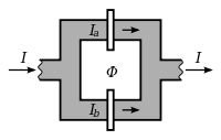


The DC SQUID was invented in 1964 by Robert Jaklevic, John J. Lambe, James Mercereau, and Arnold Silver of Ford Research Labs[3] after Brian David Josephson postulated the Josephson effect in 1962, and the first Josephson junction was made by John Rowell and Philip Anderson at Bell Labs in 1963.[4] It has two Josephson junctions in parallel in a superconducting loop. It is based on the DC Josephson effect. In the absence of any external magnetic field, the input current splits into the two branches equally. If a small external magnetic field is applied to the superconducting loop, a screening current, , begins circulating in the loop that generates a magnetic field canceling the applied external flux. The induced current is in the same direction as in one of the branches of the superconducting loop, and is opposite to in the other branch; the total current becomes in one branch and in the other. As soon as the current in either branch exceeds the critical current, , of the Josephson junction, a voltage appears across the junction.


Now suppose the external flux is further increased until it exceeds , half the magnetic flux quantum. Since the flux enclosed by the superconducting loop must be an integer number of flux quanta, instead of screening the flux the SQUID now energetically prefers to increase it to . The screening current now flows in the opposite direction. Thus the screening current changes direction every time the flux increases by half integer multiples of . Thus the critical current oscillates as a function of the applied flux. If the input current is more than , then the SQUID always operates in the resistive mode. The voltage in this case is thus a function of the applied magnetic field and the period equal to . Since the current-voltage characteristics of the DC SQUID is hysteretic, a shunt resistance, is connected across the junction to eliminate the hysteresis (in the case of copper oxide based high-temperature superconductors the junction's own intrinsic resistance is usually sufficient). The screening current is the applied flux divided by the self-inductance of the ring. Thus can be estimated as the function of (flux to voltage converter)[5][6] as follows:


- ∆V = R ∆I
- 2I = 2 ∆Φ/L, where L is the self inductance of the superconducting ring
- ∆V = (R/L) ∆Φ
The discussion in this Section assumed perfect flux quantization in the loop. However, this is only true for big loops with a large self-inductance. According to the relations, given above, this implies also small current and voltage variations. In practice the self-inductance L of the loop is not so large. The general case can be evaluated by introducing a parameter

with ic the critical current of the SQUID. Usually λ is of order one.[7]
RF SQUID

The RF SQUID was invented in 1965 by Robert Jaklevic, John J. Lambe, Arnold Silver, and James Edward Zimmerman at Ford.[6] It is based on the AC Josephson effect and uses only one Josephson junction. It is less sensitive compared to DC SQUID but is cheaper and easier to manufacture in smaller quantities. Most fundamental measurements in biomagnetism, even of extremely small signals, have been made using RF SQUIDS.[8][9] The RF SQUID is inductively coupled to a resonant tank circuit. Depending on the external magnetic field, as the SQUID operates in the resistive mode, the effective inductance of the tank circuit changes, thus changing the resonant frequency of the tank circuit. These frequency measurements can be easily taken, and thus the losses which appear as the voltage across the load resistor in the circuit are a periodic function of the applied magnetic flux with a period of Φ0. For a precise mathematical description refer to the original paper by Erné et al.[5][10]
Materials used
The traditional superconducting materials for SQUIDs are pure niobium or a lead alloy with 10% gold or indium, as pure lead is unstable when its temperature is repeatedly changed. To maintain superconductivity, the entire device needs to operate within a few degrees of absolute zero, cooled with liquid helium.
In 2006, proof of concept has be shown for CNT-SQUID sensors built with an Aluminum loop and a single walled carbon nanotube Josephson junctions.[11] The sensors is few 100 nm size and operates at 1K or below. Such sensors allow to count spins.[12]
High-temperature SQUID sensors are more recent; they are made of high-temperature superconductors, particularly YBCO, and are cooled by liquid nitrogen which is cheaper and more easily handled than liquid helium. They are less sensitive than conventional low temperature SQUIDs but good enough for many applications.
Uses

The extreme sensitivity of SQUIDs makes them ideal for studies in biology. Magnetoencephalography (MEG), for example, uses measurements from an array of SQUIDs to make inferences about neural activity inside brains. Because SQUIDs can operate at acquisition rates much higher than the highest temporal frequency of interest in the signals emitted by the brain (kHz), MEG achieves good temporal resolution. Another area where SQUIDs are used is magnetogastrography, which is concerned with recording the weak magnetic fields of the stomach. A novel application of SQUIDs is the magnetic marker monitoring method, which is used to trace the path of orally applied drugs. In the clinical environment SQUIDs are used in cardiology for magnetic field imaging (MFI), which detects the magnetic field of the heart for diagnosis and risk stratification.
Probably the most common commercial use of SQUIDs is in magnetic property measurement systems (MPMS). These are turn-key systems, made by several manufacturers, that measure the magnetic properties of a material sample. This is typically done over a temperature range from that of 300 mK to roughly 400 K.[13] With the decreasing size of SQUID sensors since the last decade, such sensor can equip the tip of an AFM probe. Such device allows simultaneous measurement of roughness of the surface of a sample and the local magnetic flux.[14]
For example, SQUIDs are being used as detectors to perform magnetic resonance imaging (MRI). While high-field MRI uses precession fields of one to several teslas, SQUID-detected MRI uses measurement fields that lie in the microtesla range. In a conventional MRI system, the signal scales as the square of the measurement frequency (and hence precession field): one power of frequency comes from the thermal polarization of the spins at ambient temperature, while the second power of field comes from the fact that the induced voltage in the pickup coil is proportional to the frequency of the precessing magnetization. In the case of untuned SQUID detection of prepolarized spins, however, the NMR signal strength is independent of precession field, allowing MRI signal detection in extremely weak fields, of order the Earth's field. SQUID-detected MRI has advantages over high-field MRI systems, such as the low cost required to build such a system, and its compactness. The principle has been demonstrated by imaging human extremities, and its future application may include tumor screening.[15]
Another application is the scanning SQUID microscope, which uses a SQUID immersed in liquid helium as the probe. The use of SQUIDs in oil prospecting, mineral exploration, earthquake prediction and geothermal energy surveying is becoming more widespread as superconductor technology develops; they are also used as precision movement sensors in a variety of scientific applications, such as the detection of gravitational waves.[16] A SQUID is the sensor in each of the four gyroscopes employed on Gravity Probe B in order to test the limits of the theory of general relativity.[1]
A modified RF SQUID was used to observe the dynamical Casimir effect for the first time.[17][18]
Proposed uses
It has also been suggested that they might be implemented in a quantum computer.[19]
A potential military application exists for use in anti-submarine warfare as a magnetic anomaly detector (MAD) fitted to maritime patrol aircraft.[20]
See also
Notes
- 1 2 Ran, Shannon K’doah (2004). Gravity Probe B: Exploring Einstein's Universe with Gyroscopes (PDF). NASA. p. 26.
- ↑ D. Drung; C. Assmann; J. Beyer; A. Kirste; M. Peters; F. Ruede & Th. Schurig (2007). "Highly sensitive and easy-to-use SQUID sensors" (PDF). IEEE Transactions on Applied Superconductivity. 17 (2): 699–704. Bibcode:2007ITAS...17..699D. doi:10.1109/TASC.2007.897403.
- ↑ R. C. Jaklevic; J. Lambe; A. H. Silver & J. E. Mercereau (1964). "Quantum Interference Effects in Josephson Tunneling". Phys. Rev. Letters. 12 (7): 159–160. Bibcode:1964PhRvL..12..159J. doi:10.1103/PhysRevLett.12.159.
- ↑ Anderson, P.; Rowell, J. (1963). "Probable Observation of the Josephson Superconducting Tunneling Effect". Physical Review Letters. 10 (6): 230–232. Bibcode:1963PhRvL..10..230A. doi:10.1103/PhysRevLett.10.230.
- 1 2 E. du Trémolet de Lacheisserie, D. Gignoux, and M. Schlenker (editors) (2005). Magnetism: Materials and Applications. 2. Springer.
- 1 2 J. Clarke and A. I. Braginski (Eds.) (2004). The SQUID handbook. 1. Wiley-Vch.
- ↑ A.TH.A.M. de Waele & R. de Bruyn Ouboter (1969). "Quantum-interference phenomena in point contacts between two superconductors". Physica. 41 (2): 225–254. Bibcode:1969Phy....41..225D. doi:10.1016/0031-8914(69)90116-5.
- ↑ Romani, G. L.; Williamson, S. J.; Kaufman, L. (1982). "Biomagnetic instrumentation". Review of Scientific Instruments. 53 (12): 1815–1845. Bibcode:1982RScI...53.1815R. doi:10.1063/1.1136907. PMID 6760371.
- ↑ Sternickel, K.; Braginski, A. I. (2006). "Biomagnetism using SQUIDs: Status and perspectives". Superconductor Science and Technology. 19 (3): S160. Bibcode:2006SuScT..19S.160S. doi:10.1088/0953-2048/19/3/024.
- ↑ S.N. Erné; H.-D. Hahlbohm; H. Lübbig (1976). "Theory of the RF biased Superconducting Quantum Interference Device for the non-hysteretic regime". J. Appl. Phys. 47 (12): 5440–5442. Bibcode:1976JAP....47.5440E. doi:10.1063/1.322574.
- ↑ Cleuziou, J.-P.; Wernsdorfer, W. (2006). "Carbon nanotube superconducting quantum interference device". Nature Nanotechnology. 1 (October): 53–9. Bibcode:2006NatNa...1...53C. doi:10.1038/nnano.2006.54. PMID 18654142.
- ↑ Aprili, Marco (2006). "The nanoSQUID makes its debut". Nature Nanotechnology. 1 (October).
- ↑ Kleiner, R.; Koelle, D.; Ludwig, F.; Clarke, J. (2004). "Superconducting quantum interference devices: State of the art and applications". Proceedings of the IEEE. 92 (10): 1534–1548. doi:10.1109/JPROC.2004.833655.
- ↑ microSQUID microscopy at Institut Néel (Grenoble, FRANCE)
- ↑ Clarke, J.; Lee, A.T.; Mück, M.; Richards, P.L. "Chapter 8.3: Nuclear Magnetic and Quadrupole Resonance and Magnetic Resonance Imaging". pp. 56–81. Missing or empty
|title=(help) in Clarke & Braginski 2006 - ↑ Paik, Ho J. "Chapter 15.2: Superconducting Transducer for Gravitational-Wave Detectors". pp. 548–554. Missing or empty
|title=(help) in Clarke & Braginski 2006 - ↑ "First Observation of the Dynamical Casimir Effect". Technology Review.
- ↑ Wilson, C. M. (2011). "Observation of the Dynamical Casimir Effect in a Superconducting Circuit". Nature. 479 (7373): 376–379. arXiv:1105.4714
 . Bibcode:2011Natur.479..376W. doi:10.1038/nature10561. PMID 22094697.
 - ↑ Quantum coherence with a single Cooper pair, V Bouchiat, D Vion, P Joyez, D Esteve, M H Devoret, 1998 Phys. Scr. 1998 165
- ↑ Ouellette, Jennifer. "SQUID Sensors Penetrate New Markets" (PDF). The Industrial Physicist. p. 22. Archived from the original (PDF) on 18 May 2008.
References
- Clarke, John; Braginski, Alex I., eds. (2006). The SQUID Handbook: Applications of SQUIDs and SQUID Systems. 2. Wiley-VCH. ISBN 978-3-527-40408-7.