Rotation formalisms in three dimensions
In geometry, various formalisms exist to express a rotation in three dimensions as a mathematical transformation. In physics, this concept is applied to classical mechanics where rotational (or angular) kinematics is the science of quantitative description of a purely rotational motion. The orientation of an object at a given instant is described with the same tools, as it is defined as an imaginary rotation from a reference placement in space, rather than an actually observed rotation from a previous placement in space.
According to Euler's rotation theorem the rotation of a rigid body (or three-dimensional coordinate system with the fixed origin) is described by a single rotation about some axis. Such a rotation may be uniquely described by a minimum of three real parameters. However, for various reasons, there are several ways to represent it. Many of these representations use more than the necessary minimum of three parameters, although each of them still has only three degrees of freedom.
An example where rotation representation is used is in computer vision, where an automated observer needs to track a target. Let's consider a rigid body, with three orthogonal unit vectors fixed to its body (representing the three axes of the object's local coordinate system). The basic problem is to specify the orientation of these three unit vectors, and hence the rigid body, with respect to the observer's coordinate system, regarded as a reference placement in space.
Rotations and motions
Rotation formalisms are focused on proper (orientation-preserving) motions of the Euclidean space with one fixed point, that a rotation refers to. Although physical motions with a fixed point are an important case (such as ones described in the center-of-mass frame, or motions of a joint), this approach creates a knowledge about all motions. Any proper motion of the Euclidean space decomposes to a rotation around the origin and a translation. Whichever the order of their composition will be, the "pure" rotation component wouldn't change, uniquely determined by the complete motion.
One can also understand "pure" rotations as linear maps in a vector space equipped with Euclidean structure, not as maps of points of a corresponding affine space. In other words, a rotation formalism captures only the rotational part of a motion, that contains three degrees of freedom, and ignores the translational part, that contains another three.
Formalism alternatives
Rotation matrix
The above-mentioned triad of unit vectors is also called a basis. Specifying the coordinates (components) of vectors of this basis in its current (rotated) position, in terms of the reference (non-rotated) coordinate axes, will completely describe the rotation. The three unit vectors, , and , that form the rotated basis each consist of 3 coordinates, yielding a total of 9 parameters.


These parameters can be written as the elements of a 3×3 matrix A, called a rotation matrix. Typically, the coordinates of each of these vectors are arranged along a column of the matrix (however, beware that an alternative definition of rotation matrix exists and is widely used, where the vectors coordinates defined above are arranged by rows[1])
![\mathbf {A} =\left[{\begin{array}{ccc}{\hat {\mathbf {u} }}_{x}&{\hat {\mathbf {v} }}_{x}&{\hat {\mathbf {w} }}_{x}\\{\hat {\mathbf {u} }}_{y}&{\hat {\mathbf {v} }}_{y}&{\hat {\mathbf {w} }}_{y}\\{\hat {\mathbf {u} }}_{z}&{\hat {\mathbf {v} }}_{z}&{\hat {\mathbf {w} }}_{z}\\\end{array}}\right]](../I/m/f6952e016f6b8d9eb3479c77dffcf566c5989f9e.svg)
The elements of the rotation matrix are not all independent—as Euler's rotation theorem dictates, the rotation matrix has only three degrees of freedom.
The rotation matrix has the following properties:
- A is a real, orthogonal matrix, hence each of its rows or columns represents a unit vector.
- The eigenvalues of A are
- where i is the standard imaginary unit with the property i2 = −1

- The determinant of A is +1, equivalent to the product of its eigenvalues.
- The trace of A is , equivalent to the sum of its eigenvalues.

The angle which appears in the eigenvalue expression corresponds to the angle of the Euler axis and angle representation. The eigenvector corresponding to the eigenvalue of 1 is the accompanying Euler axis, since the axis is the only (nonzero) vector which remains unchanged by left-multiplying (rotating) it with the rotation matrix.

The above properties are equivalent to:

which is another way of stating that form a 3D orthonormal basis. These statements comprise a total of 6 conditions (the cross product contains 3), leaving the rotation matrix with just 3 degrees of freedom, as required.

Two successive rotations represented by matrices and are easily combined as elements of a group,


(Note the order, since the vector being rotated is multiplied from the right). The ease by which vectors can be rotated using a rotation matrix, as well as the ease of combining successive rotations, make the rotation matrix a useful and popular way to represent rotations, even though it is less concise than other representations.
Euler axis and angle (rotation vector)
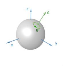
From Euler's rotation theorem we know that any rotation can be expressed as a single rotation about some axis. The axis is the unit vector (unique except for sign) which remains unchanged by the rotation. The magnitude of the angle is also unique, with its sign being determined by the sign of the rotation axis.
The axis can be represented as a three-dimensional unit vector , and the angle by a scalar .
![\scriptstyle {\hat {\mathbf {e} }}\;=\;[e_{x}\ e_{y}\ e_{z}]^{\mathrm {T} }](../I/m/474408d60afcde115afe519d9e1299d6339a248d.svg)
Since the axis is normalized, it has only two degrees of freedom. The angle adds the third degree of freedom to this rotation representation.
One may wish to express rotation as a rotation vector, or Euler vector, an un-normalized three-dimensional vector the direction of which specifies the axis, and the length of which is θ,

The rotation vector is in some contexts useful, as it represents a three-dimensional rotation with only three scalar values (its components), representing the three degrees of freedom. This is also true for representations based on sequences of three Euler angles (see below).
If the rotation angle is zero, the axis is not uniquely defined. Combining two successive rotations, each represented by an Euler axis and angle, is not straightforward, and in fact does not satisfy the law of vector addition, which shows that finite rotations are not really vectors at all. It is best to employ the rotation matrix or quaternion notation, calculate the product, and then convert back to Euler axis and angle.
Euler rotations
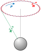
The idea behind Euler rotations is to split the complete rotation of the coordinate system into three simpler constitutive rotations, called Precession, Nutation, and intrinsic rotation, being each one of them an increment on one of the Euler angles. Notice that the outer matrix will represent a rotation around one of the axes of the reference frame, and the inner matrix represents a rotation around one of the moving frame axis. The middle matrix represent a rotation around an intermediate axis called line of nodes.
However, the definition of Euler angles is not unique and in the literature many different conventions are used. These conventions depend on the axes about which the rotations are carried out, and their sequence (since rotations are not commutative).
The convention being used is usually indicated by specifying the axes about which the consecutive rotations (before being composed) take place, referring to them by index (1, 2, 3) or letter (X, Y, Z). The engineering and robotics communities typically use 3-1-3 Euler angles. Notice that after composing the independent rotations, they do not rotate about their axis anymore. The most external matrix rotates the other two, leaving the second rotation matrix over the line of nodes, and the third one in a frame comoving with the body. There are 3×3×3 = 27 possible combinations of three basic rotations but only 3×2×2 = 12 of them can be used for representing arbitrary 3D rotations as Euler angles. These 12 combinations avoid consecutive rotations around the same axis (such as XXY) which would reduce the degrees of freedom that can be represented.
Therefore, Euler angles are never expressed in terms of the external frame, or in terms of the co-moving rotated body frame, but in a mixture. Other conventions (e.g., rotation matrix or quaternions) are used to avoid this problem.
In aviation orientation of the aircraft is usually expressed as intrinsic Tait-Bryan angles following z-y’-x″ convention, which are called heading, elevation and bank, or yaw, pitch and roll.
Quaternions
Quaternions, that form a four-dimensional vector space, have proven very useful in representing rotations due to several advantages above the other representations mentioned in this article.
A quaternion representation of rotation is written as a versor (normalized quaternion)
![{\hat {\mathbf {q} }}=\mathbf {i} q_{i}+\mathbf {j} q_{j}+\mathbf {k} q_{k}+q_{r}=[q_{i}\ q_{j}\ q_{k}\ q_{r}]^{\mathrm {T} }](../I/m/ed8255cb1391467bf453c317c79fe7e91a4a6210.svg)
The above definition stores quaternion as an array following the convention used in (Wertz 1980) and (Markley 2003). An alternative definition used for example in (Coutsias 1999) and (Schmidt 2001) defines the "scalar" term as the first quaternion element, with the other elements shifted down one position.
In terms of the Euler axis
![{\hat {\mathbf {e} }}=[e_{x}\ e_{y}\ e_{z}]^{\mathrm {T} }](../I/m/afde95c36141459fcd161099c0103778e05b4a16.svg)
and angle

this versor's components are expressed as follows:

Inspection shows that the quaternion parametrization obeys the following constraint:

The last term (in our definition) is often called the scalar term, which has its origin in quaternions when understood as the mathematical extension of the complex numbers, written as
- with


and where are the hypercomplex numbers satisfying


Quaternion multiplication, that is used to specify a composite rotation, is performed in the same manner as multiplication of complex numbers, except that the order of elements must be taken into account, since multiplication is not commutative. In matrix notation we can write quaternion multiplication as
![{\tilde {\mathbf {q} }}\otimes \mathbf {q} =\left[{\begin{array}{rrrr}q_{r}&q_{k}&-q_{j}&q_{i}\\-q_{k}&q_{r}&q_{i}&q_{j}\\q_{j}&-q_{i}&q_{r}&q_{k}\\-q_{i}&-q_{j}&-q_{k}&q_{r}\end{array}}\right]\left[{\begin{array}{c}{\tilde {q}}_{i}\\{\tilde {q}}_{j}\\{\tilde {q}}_{k}\\{\tilde {q}}_{r}\end{array}}\right]=\left[{\begin{array}{rrrr}{\tilde {q}}_{r}&-{\tilde {q}}_{k}&{\tilde {q}}_{j}&{\tilde {q}}_{i}\\{\tilde {q}}_{k}&{\tilde {q}}_{r}&-{\tilde {q}}_{i}&{\tilde {q}}_{j}\\-{\tilde {q}}_{j}&{\tilde {q}}_{i}&{\tilde {q}}_{r}&{\tilde {q}}_{k}\\-{\tilde {q}}_{i}&-{\tilde {q}}_{j}&-{\tilde {q}}_{k}&{\tilde {q}}_{r}\end{array}}\right]\left[{\begin{array}{c}q_{i}\\q_{j}\\q_{k}\\q_{r}\end{array}}\right]](../I/m/6b8aa75534a974fe4c61f01350d5f1ccef181b3b.svg)
Combining two consecutive quaternion rotations is therefore just as simple as using the rotation matrix. Remember that two successive rotation matrices, followed by , are combined as follows:

We can represent this with quaternion parameters in a similarly concise way:

Quaternions are a very popular parametrization due to the following properties:
- More compact than the matrix representation and less susceptible to round-off errors
- The quaternion elements vary continuously over the unit sphere in , (denoted by ) as the orientation changes, avoiding discontinuous jumps (inherent to three-dimensional parameterizations)
- Expression of the rotation matrix in terms of quaternion parameters involves no trigonometric functions
- It is simple to combine two individual rotations represented as quaternions using a quaternion product


Like rotation matrices, quaternions must sometimes be re-normalized due to rounding errors, to make sure that they correspond to valid rotations. The computational cost of re-normalizing a quaternion, however, is much less than for normalizing a 3×3 matrix.
Quaternions also capture the spinorial character of rotations in three dimensions. For a three-dimensional object connected to its (fixed) surroundings by slack strings or bands, the strings or bands can be untangled after two complete turns about some fixed axis from an initial untangled state. Algebraically, the quaternion describing such a rotation changes from a scalar +1 (initially), through (scalar + pseudovector) values to scalar -1 (at one full turn), through (scalar + pseudovector) values back to scalar +1 (at two full turns). This cycle repeats every 2 turns. After 2n turns (integer n > 0), without any intermediate untangling attempts, the strings/bands can be partially untangled back to the 2(n-1) turns state with each application of the same procedure used in untangling from 2 turns to 0 turns. Applying the same procedure n times will take a 2n tangled object back to the untangled or 0 turn state. The untangling process also removes any rotation-generated twisting about the strings/bands themselves. Simple 3D mechanical models can be used to illustrate these facts.
Rodrigues parameters and Gibbs representation
Rodrigues parameters can be expressed in terms of Euler axis and angle as follows,[2]

This has a discontinuity at 180° (π radians): each vector, r, with a norm of π radians represent the same rotation as −r.
Similarly, the Gibbs representation can be expressed as follows,

A rotation g followed by a rotation f in the Gibbs representation has the simple form

Today, the most straightforward way to prove this formula is in the (faithful) doublet representation, where g = tan a, etc.
The Gibbs vector has the advantage (or disadvantage, depending on context) that 180° rotations cannot be represented in it. (Even using floating point numbers that include infinity, rotation direction cannot be well-defined; for example, naively, a 180° rotation about the axis (1, 1, 0) would be (∞, ∞, 0), which is the same representation as 180° rotation about (1, 0.0001, 0).)
Modified Rodrigues parameters (MRPs) can be expressed in terms of Euler axis and angle by

The modified Rodrigues parameterization shares many characteristics with the rotation vector parametrization, including the occurrence of discontinuous jumps in the parameter space when incrementing the rotation.
Cayley–Klein parameters
See definition at Wolfram Mathworld.
Higher-dimensional analogues
Conversion formulae between formalisms
Rotation matrix ↔ Euler angles
The Euler angles can be extracted from the rotation matrix by inspecting the rotation matrix in analytical form.


Rotation matrix → Euler angles (z-x-z extrinsic)
Using the x-convention, the 3-1-3 extrinsic Euler angles , and (around the , and again the -axis) can be obtained as follows:


Note that is equivalent to where it also takes into account the quadrant that the point is in; see atan2.


When implementing the conversion, one has to take into account several situations:[3]
- There are generally two solutions in (−π, π]3 interval. The above formula works only when is from the interval [0, π)3.
- For special case , shall be derived from .
- There is infinitely many but countably many solutions outside of interval (−π, π]3.
- Whether all mathematical solutions apply for given application depends on the situation.


Euler angles ( z-y’-x″ intrinsic) → Rotation matrix
The rotation matrix is generated from the 3-2-1 intrinsic Euler angles by multiplying the three matrices generated by rotations about the axes.

The axes of the rotation depend on the specific convention being used. For the x-convention the rotations are about the , and axes with angles , and , the individual matrices are as follows:

![{\begin{aligned}\mathbf {A} _{X}&=\left[{\begin{array}{ccc}1&0&0\\0&\cos \phi &\sin \phi \\0&-\sin \phi &\cos \phi \end{array}}\right]\\\mathbf {A} _{Y}&=\left[{\begin{array}{ccc}\cos \theta &0&-\sin \theta \\0&1&0\\\sin \theta &0&\cos \theta \end{array}}\right]\\\mathbf {A} _{Z}&=\left[{\begin{array}{ccc}\cos \psi &\sin \psi &0\\-\sin \psi &\cos \psi &0\\0&0&1\end{array}}\right]\end{aligned}}](../I/m/8c571e2a467f1a22764a4bb56f31db8fd1c4c332.svg)
This yields

Note: This is valid for a right-hand system, which is the convention used in almost all engineering and physics disciplines.
Rotation matrix ↔ Euler axis/angle
If the Euler angle is not a multiple of , the Euler axis and angle can be computed from the elements of the rotation matrix as follows:

![\scriptstyle {\hat {\mathbf {e} }}\;=\;[e_{1}\ e_{2}\ e_{3}]^{\mathrm {T} }](../I/m/3c0556590a889069f635235526834932a39c2cd1.svg)
![{\begin{aligned}\theta &=\arccos \left({\frac {1}{2}}[A_{11}+A_{22}+A_{33}-1]\right)\\e_{1}&={\frac {A_{32}-A_{23}}{2\sin \theta }}\\e_{2}&={\frac {A_{13}-A_{31}}{2\sin \theta }}\\e_{3}&={\frac {A_{21}-A_{12}}{2\sin \theta }}\end{aligned}}](../I/m/ffb64389c7b4ecb01fb2a09c55892abcc865a267.svg)
Alternatively, the following method can be used:
Eigen-decomposition of the rotation matrix yields the eigenvalues 1, and . The Euler axis is the eigenvector corresponding to the eigenvalue of 1, and the can be computed from the remaining eigenvalues.

The Euler axis can be also found using Singular Value Decomposition since it is the normalized vector spanning the null-space of the matrix .

To convert the other way the rotation matrix corresponding to an Euler axis and angle can be computed according to the Rodrigues' rotation formula (with appropriate modification) as follows:
![\mathbf {A} =\mathbf {I} _{3}\cos \theta +(1-\cos \theta ){\hat {\mathbf {e} }}{\hat {\mathbf {e} }}^{\mathrm {T} }+[{\hat {\mathbf {e} }}]_{\times }\sin \theta](../I/m/7116988787d1f538da81bf92f99fd23e527a343f.svg)
with the 3×3 identity matrix, and

![[{\hat {\mathbf {e} }}]_{\times }=\left[{\begin{array}{ccc}0&-e_{3}&e_{2}\\e_{3}&0&-e_{1}\\-e_{2}&e_{1}&0\end{array}}\right]](../I/m/f59bd72f9f4abacacde215bdeeaa225e7eeab3b6.svg)
is the cross-product matrix.
This expands to...


Rotation matrix ↔ quaternion
When computing a quaternion from the rotation matrix there is a sign ambiguity, since and represent the same rotation.


One way of computing the quaternion from the rotation matrix is as follows:
![\scriptstyle \mathbf {q} \;=\;[q_{i}\ q_{j}\ q_{k}\ q_{r}]^{\mathrm {T} }=\mathbf {i} q_{i}+\mathbf {j} q_{j}+\mathbf {k} q_{k}+q_{r}](../I/m/3d6b95bca680dfa6d000b97b3bedc4484cd926cf.svg)

There are three other mathematically equivalent ways to compute . Numerical inaccuracy can be reduced by avoiding situations in which the denominator is close to zero. One of the other three methods looks as follows:[4]

The rotation matrix corresponding to the quaternion can be computed as follows:

with the 3×3 identity matrix, and
![{\check {\mathbf {q} }}=\left[{\begin{array}{c}q_{i}\\q_{j}\\q_{k}\end{array}}\right],\ \ \ \mathbf {\mathcal {Q}} =\left[{\begin{array}{ccc}0&-q_{k}&q_{j}\\q_{k}&0&-q_{i}\\-q_{j}&q_{i}&0\end{array}}\right]](../I/m/442aada9d3128aa4425c8bcf72a9caf4871b74b3.svg)
which gives
![\mathbf {A} =\left[{\begin{array}{ccc}1-2q_{j}^{2}-2q_{k}^{2}&2(q_{i}q_{j}-q_{k}q_{r})&2(q_{i}q_{k}+q_{j}q_{r})\\2(q_{i}q_{j}+q_{k}q_{r})&1-2q_{i}^{2}-2q_{k}^{2}&2(q_{j}q_{k}-q_{i}q_{r})\\2(q_{i}q_{k}-q_{j}q_{r})&2(q_{i}q_{r}+q_{j}q_{k})&1-2q_{i}^{2}-2q_{j}^{2}\end{array}}\right]](../I/m/025c788df100bd2753d608904d1e254d2e67d09e.svg)
or equivalently
![\mathbf {A} =\left[{\begin{array}{ccc}-1+2q_{i}^{2}+2q_{r}^{2}&2(q_{i}q_{j}-q_{k}q_{r})&2(q_{i}q_{k}+q_{j}q_{r})\\2(q_{i}q_{j}+q_{k}q_{r})&-1+2q_{j}^{2}+2q_{r}^{2}&2(q_{j}q_{k}-q_{i}q_{r})\\2(q_{i}q_{k}-q_{j}q_{r})&2(q_{i}q_{r}+q_{j}q_{k})&-1+2q_{k}^{2}+2q_{r}^{2}\end{array}}\right]](../I/m/814dbdb9fb8595c219739350958b8b0a93d201e6.svg)
Euler angles ↔ Quaternion
Euler angles (z-x-z extrinsic) → Quaternion
We will consider the x-convention 3-1-3 extrinsic Euler Angles for the following algorithm. The terms of the algorithm depend on the convention used.
We can compute the quaternion from the Euler angles as follows:
![\scriptstyle \mathbf {q} =[q_{i}\ q_{j}\ q_{k}\ q_{r}]^{\mathrm {T} }=\mathbf {i} q_{i}+\mathbf {j} q_{j}+\mathbf {k} q_{k}+q_{r}](../I/m/adafdc499e238039089e361593b139f826b0a81a.svg)

Euler angles (z-y’-x″ intrinsic) → Quaternion
Quaternion equivalent to yaw (), pitch () and roll () angles or intrinsic Tait-Bryan angles following z-y’-x″ convention, can be computed by


Quaternion → Euler angles (z-x-z extrinsic)
Given the rotation quaternion , the x-convention 3-1-3 extrinsic Euler Angles can be computed by

Quaternion → Euler angles (z-y’-x″ intrinsic)
Given the rotation quaternion , yaw, pitch and roll angles or intrinsic Tait-Bryan angles following z-y’-x″ convention, can be computed by


Euler axis/angle ↔ quaternion
Given the Euler axis and angle , the quaternion

![\mathbf {q} =[q_{i}\ q_{j}\ q_{k}\ q_{r}]^{\mathrm {T} }=\mathbf {i} q_{i}+\mathbf {j} q_{j}+\mathbf {k} q_{k}+q_{r}](../I/m/edceb7853e82905f57dc67bfd68283929972cab6.svg)
can be computed by

Given the rotation quaternion , define . Then the Euler axis and angle can be computed by
![\scriptstyle {\check {\mathbf {q} }}\;=\;[q_{i}\ q_{j}\ q_{k}]^{\mathrm {T} }](../I/m/c780473680df6e300de32d387bc6cbce376fb10e.svg)

Conversion formulae for derivatives
Rotation matrix ↔ angular velocities
The angular velocity vector can be extracted from the derivative of the rotation matrix by the following relation:


![[\mathbf {\omega } ]_{\times }=\left[{\begin{array}{ccc}0&-\omega _{z}&\omega _{y}\\\omega _{z}&0&-\omega _{x}\\-\omega _{y}&\omega _{x}&0\end{array}}\right]={\frac {d\mathbf {A} }{dt}}\mathbf {A} ^{\mathrm {T} }](../I/m/5c87b036c199b81a5f1bf28e3d969e3dfe9627a5.svg)
The derivation is adapted from [5] as follows:
For any vector consider and differentiate it:


The derivative of a vector is the linear velocity of its tip. Since A is a rotation matrix, by definition the length of is always equal to the length of , and hence it does not change with time. Thus, when rotates, its tip moves along a circle, and the linear velocity of its tip is tangential to the circle; i.e., always perpendicular to . In this specific case, the relationship between the linear velocity vector and the angular velocity vector is

- (see circular motion and Cross product).
![{\frac {dr}{dt}}=\mathbf {\omega } (t)\times r(t)=[\mathbf {\omega } ]_{\times }r(t)](../I/m/c217120ecba8ae5a4a791ecc7a982e8b81ab5c2d.svg)
By the transitivity of the above-mentioned equations,
![{\frac {d\mathbf {A} }{dt}}\mathbf {A} ^{\mathrm {T} }(t)r(t)=[\mathbf {\omega } ]_{\times }r(t)](../I/m/1c647313e4b958f88c09f2d9e79f0bf463df20a6.svg)
which implies (Q.E.D.),
![{\frac {d\mathbf {A} }{dt}}\mathbf {A} ^{\mathrm {T} }(t)=[\mathbf {\omega } ]_{\times }](../I/m/e1734e25df76ab7f9e5392203ee8d80cb5582154.svg)
Quaternion ↔ angular velocities
The angular velocity vector can be obtained from the derivative of the quaternion as follows:[6]

![\left[ {\begin{array}{c}
\omega_x \\
\omega_y \\
\omega_z \\
0
\end{array}} \right] = 2 \frac{d\mathbf{q}}{dt} \otimes \tilde{\mathbf{q}}](../I/m/07095998d6cc17ed86c6cb4503dbad3192166911.svg)
where is the inverse of .


Conversely, the derivative of the quaternion is
![{\displaystyle {\frac {d\mathbf {q} }{dt}}={\frac {1}{2}}\left[{\begin{array}{c}\omega _{x}\\\omega _{y}\\\omega _{z}\\0\end{array}}\right]\otimes \mathbf {q} }](../I/m/c82565c70d084243b094fcfa539587594e7fd2ed.svg)
Rotors in a geometric algebra
The formalism of geometric algebra (GA) provides an extension and interpretation of the quaternion method. Central to GA is the geometric product of vectors, an extension of the traditional inner and cross products, given by

where the symbol denotes the outer product. This product of vectors produces two terms: a scalar part from the inner product and a bivector part from the outer product. This bivector describes the plane perpendicular to what the cross product of the vectors would return.


Bivectors in GA have some unusual properties compared to vectors. Under the geometric product, bivectors have negative square: the bivector describes the -plane. Its square is . Because the unit basis vectors are orthogonal to each other, the geometric product reduces to the antisymmetric outer product – and can be swapped freely at the cost of a factor of −1. The square reduces to since the basis vectors themselves square to +1.


This result holds generally for all bivectors, and as a result the bivector plays a role similar to the imaginary unit. Geometric algebra uses bivectors in its analogue to the quaternion, the rotor, given by , where is a unit bivector that describes the plane of rotation. Because squares to −1, the power series expansion of generates the trigonometric functions. The rotation formula that maps a vector to a rotated vector is then


where is the reverse of (reversing the order of the vectors in is equivalent to changing its sign).


Example. A rotation about the axis can be accomplished by converting to its dual bivector, , where is the unit volume element, the only trivector (pseudoscalar) in three-dimensional space. The result is . In three-dimensional space, however, it is often simpler to leave the expression for , using the fact that commutes with all objects in 3D and also squares to −1. A rotation of the vector in this plane by an angle is then


Recognizing that and that is the reflection of about the plane perpendicular to gives a geometric interpretation to the rotation operation: the rotation preserves the components that are parallel to and changes only those that are perpendicular. The terms are then computed:


The result of the rotation is then

A simple check on this result is the angle . Such a rotation should map the to . Indeed, the rotation reduces to


exactly as expected. This rotation formula is valid not only for vectors but for any multivector. In addition, when Euler angles are used, the complexity of the operation is much reduced. Compounded rotations come from multiplying the rotors, so the total rotor from Euler angles is

but and . These rotors come back out of the exponentials like so:


where refers to rotation in the original coordinates. Similarly for the rotation, . Noting that and commute (rotations in the same plane must commute), and the total rotor becomes


Thus, the compounded rotations of Euler angles become a series of equivalent rotations in the original fixed frame.
While rotors in geometric algebra work almost identically to quaternions in three dimensions, the power of this formalism is its generality: this method is appropriate and valid in spaces with any number of dimensions. In 3D, rotations have three degrees of freedom, a degree for each linearly independent plane (bivector) the rotation can take place in. It has been known that pairs of quaternions can be used to generate rotations in 4D, yielding six degrees of freedom, and the geometric algebra approach verifies this result: in 4D, there are six linearly independent bivectors that can be used as the generators of rotations.
See also
- Euler filter
- Orientation (geometry)
- Rotation around a fixed axis
- Three-dimensional rotation operator
References
- ↑ Rotation Matrix, http://mathworld.wolfram.com/RotationMatrix.html
- ↑ cf. J Willard Gibbs (1884). Elements of Vector Analysis, New Haven, p. 67
- ↑ Direct and inverse kinematics lecture notes, page 5
- ↑ Mebius, Johan (2007). "Derivation of the Euler–Rodrigues formula for three-dimensional rotations from the general formula for four-dimensional rotations". arXiv:math/0701759
 .
. - ↑ Physics - Mark Ioffe - W(t) in terms of matrices
- ↑ Physics - Kinematics - Angular Velocity
- Evangelos A. Coutsias and Louis Romero, (1999) The Quaternions with an application to Rigid Body Dynamics, Department of Mathematics and Statistics, University of New Mexico.
- F. Landis Markley, (2003) Attitude Error Representations for Kalman Filtering, Journal of Guidance, Control and Dynamics.
- H. Goldstein, (1980) Classical Mechanics, 2nd. ed., Addison–Wesley. ISBN 0-201-02918-9
- James R. Wertz, (1980) Spacecraft Attitude Determination and Control, D. Reidel Publishing Company. ISBN 90-277-1204-2
- J. Schmidt and H. Niemann, (2001) Using Quaternions for Parametrizing 3-D Rotations in Unconstrained Nonlinear Optimization, Vision, Modeling and Visualization (VMV01).
- Lev D. Landau and E. M. Lifshitz, (1976) Mechanics, 3rd. ed., Pergamon Press. ISBN 0-08-021022-8 (hardcover) and ISBN 0-08-029141-4 (softcover).
- Klumpp, A. R., Singularity-Free Extraction of a Quaternion from a Direction-Cosine Matrix, Journal of Spacecraft and Rockets, vol. 13, Dec. 1976, p. 754, 755.
- C. Doran and A. Lasenby, (2003) Geometric Algebra for Physicists, Cambridge University Press. ISBN 978-0-521-71595-9
External links
- EuclideanSpace has a wealth of information on rotation representation
- Q36. How do I generate a rotation matrix from Euler angles? and Q37. How do I convert a rotation matrix to Euler angles? — The Matrix and Quaternions FAQ
- Imaginary numbers are not Real – the Geometric Algebra of Spacetime – Section "Rotations and Geometric Algebra" derives and applies the rotor description of rotations
- Starlino's DCM Tutorial – Direction cosine matrix theory tutorial and applications. Space orientation estimation algorithm using accelerometer, gyroscope and magnetometer IMU devices. Using complimentary filter (popular alternative to Kalman filter) with DCM matrix.