Robust regression
| Part of a series on Statistics |
| Regression analysis |
|---|
 |
| Models |
| Estimation |
| Background |
|
In robust statistics, robust regression is a form of regression analysis designed to circumvent some limitations of traditional parametric and non-parametric methods. Regression analysis seeks to find the relationship between one or more independent variables and a dependent variable. Certain widely used methods of regression, such as ordinary least squares, have favourable properties if their underlying assumptions are true, but can give misleading results if those assumptions are not true; thus ordinary least squares is said to be not robust to violations of its assumptions. Robust regression methods are designed to be not overly affected by violations of assumptions by the underlying data-generating process.
In particular, least squares estimates for regression models are highly sensitive to (not robust against) outliers. While there is no precise definition of an outlier, outliers are observations which do not follow the pattern of the other observations. This is not normally a problem if the outlier is simply an extreme observation drawn from the tail of a normal distribution, but if the outlier results from non-normal measurement error or some other violation of standard ordinary least squares assumptions, then it compromises the validity of the regression results if a non-robust regression technique is used.
Applications
Heteroscedastic errors
One instance in which robust estimation should be considered is when there is a strong suspicion of heteroscedasticity. In the homoscedastic model, it is assumed that the variance of the error term is constant for all values of x. Heteroscedasticity allows the variance to be dependent on x, which is more accurate for many real scenarios. For example, the variance of expenditure is often larger for individuals with higher income than for individuals with lower incomes. Software packages usually default to a homoscedastic model, even though such a model may be less accurate than a heteroscedastic model. One simple approach (Tofallis, 2008) is to apply least squares to percentage errors as this reduces the influence of the larger values of the dependent variable compared to ordinary least squares.
Presence of outliers
Another common situation in which robust estimation is used occurs when the data contain outliers. In the presence of outliers that do not come from the same data-generating process as the rest of the data, least squares estimation is inefficient and can be biased. Because the least squares predictions are dragged towards the outliers, and because the variance of the estimates is artificially inflated, the result is that outliers can be masked. (In many situations, including some areas of geostatistics and medical statistics, it is precisely the outliers that are of interest.)
Although it is sometimes claimed that least squares (or classical statistical methods in general) are robust, they are only robust in the sense that the type I error rate does not increase under violations of the model. In fact, the type I error rate tends to be lower than the nominal level when outliers are present, and there is often a dramatic increase in the type II error rate. The reduction of the type I error rate has been labelled as the conservatism of classical methods.
History and unpopularity of robust regression
Despite their superior performance over least squares estimation in many situations, robust methods for regression are still not widely used. Several reasons may help explain their unpopularity (Hampel et al. 1986, 2005). One possible reason is that there are several competing methods and the field got off to many false starts. Also, computation of robust estimates is much more computationally intensive than least squares estimation; in recent years however, this objection has become less relevant as computing power has increased greatly. Another reason may be that some popular statistical software packages failed to implement the methods (Stromberg, 2004). The belief of many statisticians that classical methods are robust may be another reason.
Although uptake of robust methods has been slow, modern mainstream statistics text books often include discussion of these methods (for example, the books by Seber and Lee, and by Faraway; for a good general description of how the various robust regression methods developed from one another see Andersen's book). Also, modern statistical software packages such as R, Statsmodels, Stata and S-PLUS include considerable functionality for robust estimation (see, for example, the books by Venables and Ripley, and by Maronna et al.).
Methods for robust regression
Least squares alternatives
The simplest methods of estimating parameters in a regression model that are less sensitive to outliers than the least squares estimates, is to use least absolute deviations. Even then, gross outliers can still have a considerable impact on the model, motivating research into even more robust approaches.
In 1973, Huber introduced M-estimation for regression. The M in M-estimation stands for "maximum likelihood type". The method is robust to outliers in the response variable, but turned out not to be resistant to outliers in the explanatory variables (leverage points). In fact, when there are outliers in the explanatory variables, the method has no advantage over least squares.
In the 1980s, several alternatives to M-estimation were proposed as attempts to overcome the lack of resistance. See the book by Rousseeuw and Leroy for a very practical review. Least trimmed squares (LTS) is a viable alternative and is currently (2007) the preferred choice of Rousseeuw and Ryan (1997, 2008). The Theil–Sen estimator has a lower breakdown point than LTS but is statistically efficient and popular. Another proposed solution was S-estimation. This method finds a line (plane or hyperplane) that minimizes a robust estimate of the scale (from which the method gets the S in its name) of the residuals. This method is highly resistant to leverage points, and is robust to outliers in the response. However, this method was also found to be inefficient.
MM-estimation attempts to retain the robustness and resistance of S-estimation, whilst gaining the efficiency of M-estimation. The method proceeds by finding a highly robust and resistant S-estimate that minimizes an M-estimate of the scale of the residuals (the first M in the method's name). The estimated scale is then held constant whilst a close-by M-estimate of the parameters is located (the second M).
Parametric alternatives
Another approach to robust estimation of regression models is to replace the normal distribution with a heavy-tailed distribution. A t-distribution with between 4 and 6 degrees of freedom has been reported to be a good choice in various practical situations. Bayesian robust regression, being fully parametric, relies heavily on such distributions.
Under the assumption of t-distributed residuals, the distribution is a location-scale family. That is, . The degrees of freedom of the t-distribution is sometimes called the kurtosis parameter. Lange, Little and Taylor (1989) discuss this model in some depth from a non-Bayesian point of view. A Bayesian account appears in Gelman et al. (2003).

An alternative parametric approach is to assume that the residuals follow a mixture of normal distributions; in particular, a contaminated normal distribution in which the majority of observations are from a specified normal distribution, but a small proportion are from a normal distribution with much higher variance. That is, residuals have probability of coming from a normal distribution with variance , where is small, and probability of coming from a normal distribution with variance for some


Typically, . This is sometimes called the -contamination model.

Parametric approaches have the advantage that likelihood theory provides an 'off the shelf' approach to inference (although for mixture models such as the -contamination model, the usual regularity conditions might not apply), and it is possible to build simulation models from the fit. However, such parametric models still assume that the underlying model is literally true. As such, they do not account for skewed residual distributions or finite observation precisions.
Unit weights
Another robust method is the use of unit weights (Wainer & Thissen, 1976), a method that can be applied when there are multiple predictors of a single outcome. Ernest Burgess (1928) used unit weights to predict success on parole. He scored 21 positive factors as present (e.g., "no prior arrest" = 1) or absent ("prior arrest" = 0), then summed to yield a predictor score, which was shown to be a useful predictor of parole success. Samuel S. Wilks (1938) showed that nearly all sets of regression weights sum to composites that are very highly correlated with one another, including unit weights, a result referred to as Wilk's theorem (Ree, Carretta, & Earles, 1998). Robyn Dawes (1979) examined decision making in applied settings, showing that simple models with unit weights often outperformed human experts. Bobko, Roth, and Buster (2007) reviewed the literature on unit weights, and they concluded that decades of empirical studies show that unit weights perform similar to ordinary regression weights on cross validation.
Example: BUPA liver data
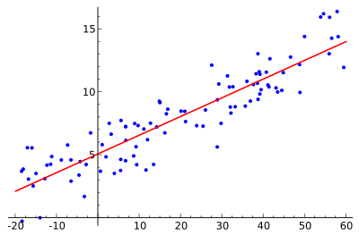
The BUPA liver data have been studied by various authors, including Breiman (2001). The data can be found via the classic data sets page and there is some discussion in the article on the Box-Cox transformation. A plot of the logs of ALT versus the logs of γGT appears below. The two regression lines are those estimated by ordinary least squares (OLS) and by robust MM-estimation. The analysis was performed in R using software made available by Venables and Ripley (2002).

The two regression lines appear to be very similar (and this is not unusual in a data set of this size). However, the advantage of the robust approach comes to light when the estimates of residual scale are considered. For ordinary least squares, the estimate of scale is 0.420, compared to 0.373 for the robust method. Thus, the relative efficiency of ordinary least squares to MM-estimation in this example is 1.266. This inefficiency leads to loss of power in hypothesis tests, and to unnecessarily wide confidence intervals on estimated parameters.
Outlier detection
Another consequence of the inefficiency of the ordinary least squares fit is that several outliers are masked. Because the estimate of residual scale is inflated, the scaled residuals are pushed closer to zero than when a more appropriate estimate of scale is used. The plots of the scaled residuals from the two models appear below. The variable on the x-axis is just the observation number as it appeared in the data set. Rousseeuw and Leroy (1986) contains many such plots.

The horizontal reference lines are at 2 and -2 so that any observed scaled residual beyond these boundaries can be considered to be an outlier. Clearly, the least squares method leads to many interesting observations being masked.
Whilst in one or two dimensions outlier detection using classical methods can be performed manually, with large data sets and in high dimensions the problem of masking can make identification of many outliers impossible. Robust methods automatically detect these observations, offering a serious advantage over classical methods when outliers are present.
See also
- RANSAC
- M-estimator
- Relaxed intersection
- Theil–Sen estimator, a method for robust simple linear regression
References
- Andersen, R. (2008). Modern Methods for Robust Regression. Sage University Paper Series on Quantitative Applications in the Social Sciences, 07-152.
- Ben-Gal I., Outlier detection, In: Maimon O. and Rockach L. (Eds.) Data Mining and Knowledge Discovery Handbook: A Complete Guide for Practitioners and Researchers," Kluwer Academic Publishers, 2005, ISBN 0-387-24435-2.
- Bobko, P., Roth, P. L., & Buster, M. A. (2007). "The usefulness of unit weights in creating composite scores: A literature review, application to content validity, and meta-analysis". Organizational Research Methods, volume 10, pages 689-709. doi:10.1177/1094428106294734
- Breiman, L. (2001). "Statistical Modeling: the Two Cultures". Statistical Science. 16 (3): 199–231. doi:10.1214/ss/1009213725. JSTOR 2676681.
- Burgess, E. W. (1928). "Factors determining success or failure on parole". In A. A. Bruce (Ed.), The Workings of the Indeterminate Sentence Law and Parole in Illinois (pp. 205–249). Springfield, Illinois: Illinois State Parole Board. Google books
- Dawes, Robyn M. (1979). "The robust beauty of improper linear models in decision making". American Psychologist, volume 34, pages 571-582. doi:10.1037/0003-066X.34.7.571 . archived pdf
- Draper, David (1988). "Rank-Based Robust Analysis of Linear Models. I. Exposition and Review". Statistical Science. 3 (2): 239–257. doi:10.1214/ss/1177012915. JSTOR 2245578.
- Faraway, J. J. (2004). Linear Models with R. Chapman & Hall/CRC.
- Fornalski, K. W. (2015). "Applications of the robust Bayesian regression analysis". International Journal of Society Systems Science. 7 (4): 314–333. doi:10.1504/IJSSS.2015.073223.
- Gelman, A.; J. B. Carlin; H. S. Stern; D. B. Rubin (2003). Bayesian Data Analysis (Second ed.). Chapman & Hall/CRC.
- Hampel, F. R.; E. M. Ronchetti; P. J. Rousseeuw; W. A. Stahel (2005) [1986]. Robust Statistics: The Approach Based on Influence Functions. Wiley.
- Lange, K. L.; R. J. A. Little; J. M. G. Taylor (1989). "Robust statistical modeling using the t-distribution". Journal of the American Statistical Association. 84 (408): 881–896. doi:10.2307/2290063. JSTOR 2290063.
- Lerman, G.; McCoy, M.; Tropp, J. A.; Zhang T. (2012). "Robust computation of linear models, or how to find a needle in a haystack", arXiv:1202.4044.
- Maronna, R.; D. Martin; V. Yohai (2006). Robust Statistics: Theory and Methods. Wiley.
- McKean, Joseph W. (2004). "Robust Analysis of Linear Models". Statistical Science. 19 (4): 562–570. doi:10.1214/088342304000000549. JSTOR 4144426.
- Radchenko S.G. (2005). Robust methods for statistical models estimation: Monograph. (on russian language). Кiev: РР «Sanspariel» ISBN 966-96574-0-7. p. 504.
- Ree, M. J., Carretta, T. R., & Earles, J. A. (1998). "In top-down decisions, weighting variables does not matter: A consequence of Wilk's theorem. Organizational Research Methods, volume 1(4), pages 407-420. doi:10.1177/109442819814003
- Rousseeuw, P. J.; A. M. Leroy (2003) [1986]. Robust Regression and Outlier Detection. Wiley.
- Ryan, T. P. (2008) [1997]. Modern Regression Methods. Wiley.
- Seber, G. A. F.; A. J. Lee (2003). Linear Regression Analysis (Second ed.). Wiley.
- Stromberg, A. J. (2004). "Why write statistical software? The case of robust statistical methods". Journal of Statistical Software.
- Strutz, T. (2016). Data Fitting and Uncertainty (A practical introduction to weighted least squares and beyond). Springer Vieweg. ISBN 978-3-658-11455-8.
- Tofallis, Chris (2008). "Least Squares Percentage Regression". Journal of Modern Applied Statistical Methods. 7: 526–534. doi:10.2139/ssrn.1406472.
- Venables, W. N.; B. D. Ripley (2002). Modern Applied Statistics with S. Springer.
- Wainer, H., & Thissen, D. (1976). "Three steps toward robust regression." Psychometrika, volume 41(1), pages 9–34. doi:10.1007/BF02291695
- Wilks, S. S. (1938). "Weighting systems for linear functions of correlated variables when there is no dependent variable". Psychometrika, volume 3, pages 23–40. doi:10.1007/BF02287917
External links
- R programming wikibooks
- Brian Ripley's robust statistics course notes.
- Nick Fieller's course notes on Statistical Modelling and Computation contain material on robust regression.
- Olfa Nasraoui's Overview of Robust Statistics
- Olfa Nasraoui's Overview of Robust Clustering
- Why write statistical software? The case of robust statistical methods, A. J. Stromberg
| |||||||||||||||||||||||||||||||||||||||||||||
| |||||||||||||||||||||||||||||||||||||||||||||
| |||||||||||||||||||||||||||||||||||||||||||||
| |||||||||||||||||||||||||||||||||||||||||||||
| |||||||||||||||||||||||||||||||||||||||||||||
| |||||||||||||||||||||||||||||||||||||||||||||
| |||||||||||||||||||||||||||||||||||||||||||||