Calibration of radiocarbon dates
Radiocarbon dating measurements produce ages in "radiocarbon years", which must be converted to calendar ages by a process called calibration. Calibration is needed because the atmospheric 14
C/12
C ratio, which is a key element in calculating radiocarbon ages, has not been constant historically.[1] Although Willard Libby, the inventor of radiocarbon dating, had pointed out as early as 1955 the possibility that the 14
C/12
C ratio might have varied over time, it was not until discrepancies began to accumulate between measured ages and known historical dates for artefacts that it became clear that a correction would need to be applied to radiocarbon ages to obtain calendar dates.[2] Radiocarbon years ago may be abbreviated 14
Cya (years ago).[3] A general term used reflecting evidence from any method is Before Present (BP).
Construction of a curve
To produce a curve that can be used to relate calendar years to radiocarbon years, a sequence of securely dated samples is needed which can be tested to determine their radiocarbon age. The study of tree rings led to the first such sequence: tree rings from individual pieces of wood show characteristic sequences of rings that vary in thickness because of environmental factors such as the amount of rainfall in a given year. These factors affect all trees in an area, so examining tree-ring sequences from old wood allows the identification of overlapping sequences. In this way, an uninterrupted sequence of tree rings can be extended far into the past. The first such published sequence, based on bristlecone pine tree rings, was created in the 1960s by Wesley Ferguson.[5] Hans Suess used this data to publish the first calibration curve for radiocarbon dating in 1967.[2][6][7] The curve showed two types of variation from the straight line: a long term fluctuation with a period of about 9,000 years, and a shorter term variation, often referred to as "wiggles", with a period of decades. Suess said he drew the line showing the wiggles by "cosmic schwung" – freehand, in other words. It was unclear for some time whether the wiggles were real or not, but they are now well-established.[6][7]
The calibration method also assumes that the temporal variation in 14
C level is global, such that a small number of samples from a specific year are sufficient for calibration. This was experimentally verified in the 1980s.[2]
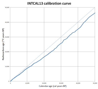
Over the next thirty years many calibration curves were published using a variety of methods and statistical approaches.[8] These were superseded by the INTCAL series of curves, beginning with INTCAL98, published in 1998, and updated in 2004, 2009, and, most recently, 2013. The improvements to these curves are based on new data gathered from tree rings, varves, coral, and other studies. Significant additions to the datasets used for INTCAL13 include non-varved marine foraminifera data, and U-Th dated speleothems. The INTCAL13 data includes separate curves for the northern and southern hemispheres, as they differ systematically because of the hemisphere effect; there is also a separate marine calibration curve.[9]

Once testing has produced a sample age in radiocarbon years, with an associated error range of plus or minus one standard deviation (usually written as ±σ), the calibration curve can be used to derive a range of calendar ages for the sample. The calibration curve itself has an associated error term, which can be seen on the graph labelled "Calibration error and measurement error". This graph shows INTCAL13 data for the calendar years 3100 BP to 3500 BP. The solid line is the INTCAL13 calibration curve, and the dotted lines show the standard error range—as with the sample error, this is one standard deviation. Simply reading off the range of radiocarbon years against the dotted lines, as is shown for sample t2, in red, gives too large a range of calendar years. The error term should be the root of the sum of the squares of the two errors:[10]

Example t1, in green on the graph, shows this procedure—the resulting error term, σtotal, is used for the range, and this range is used to read the result directly from the graph itself, without reference to the lines showing the calibration error.[10]

Variations in the calibration curve can lead to very different resulting calendar year ranges for samples with different radiocarbon ages. The graph to the right shows the part of the INTCAL13 calibration curve from 1000 BP to 1400 BP, a range in which there are significant departures from a linear relationship between radiocarbon age and calendar age. In places where the calibration curve is steep, and does not change direction, as in example t1 in blue on the graph to the right, the resulting calendar year range is quite narrow. Where the curve varies significantly both up and down, a single radiocarbon date range may produce two or more separate calendar year ranges. Example t2, in red on the graph, shows this situation: a radiocarbon age range of about 1260 BP to 1280 BP converts to three separate ranges between about 1190 BP and 1260 BP. A third possibility is that the curve is flat for some range of calendar dates; in this case, illustrated by t3, in green on the graph, a range of about 30 radiocarbon years, from 1180 BP to 1210 BP, results in a calendar year range of about a century, from 1080 BP to 1180 BP.[8]
Probabilistic methods
The method of deriving a calendar year range described above depends solely on the position of the intercepts on the graph. These are taken to be the boundaries of the 68% confidence range, or one standard deviation. However, this method does not make use of the assumption that the original radiocarbon age range is a normally distributed variable: not all dates in the radiocarbon age range are equally likely, and so not all dates in the resulting calendar year age are equally likely. Deriving a calendar year range by means of intercepts does not take this into account.[8]
The alternative is to take the original normal distribution of radiocarbon age ranges and use it to generate a histogram showing the relative probabilities for calendar ages. This has to be done by numerical methods rather than by a formula because the calibration curve is not describable as a formula.[8] Programs to perform these calculations include OxCal and CALIB. These can be accessed online; they allow the user to enter a date range at one standard deviation confidence for the radiocarbon ages, select a calibration curve, and produce probabilistic output both as tabular data and in graphical form.[11][12]
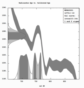
In the example CALIB output shown at left, the input data is 1270 BP, with a standard deviation of 10 radiocarbon years. The curve selected is the northern hemisphere INTCAL13 curve, part of which is shown in the output; the vertical width of the curve corresponds to the width of the standard error in the calibration curve at that point. A normal distribution is shown at left; this is the input data, in radiocarbon years. The central darker part of the normal curve is the range within one standard deviation of the mean; the lighter grey area shows the range within two standard deviations of the mean. The output is along the bottom axis; it is a trimodal graph, with peaks at around 710 AD, 740 AD, and 760 AD. Again, the ranges within the 1σ confidence range are in dark grey, and the ranges within the 2σ confidence range are in light grey. This output can be compared with the output of the intercept method in the graph above for the same radiocarbon date range.[12]
For a set of samples with a known sequence and separation in time such as a sequence of tree rings, the samples' radiocarbon ages form a small subset of the calibration curve. The resulting curve can then be matched to the actual calibration curve by identifying where, in the range suggested by the radiocarbon dates, the wiggles in the calibration curve best match the wiggles in the curve of sample dates. This "wiggle-matching" technique can lead to more precise dating than is possible with individual radiocarbon dates.[13] Since the data points on the calibration curve are five years or more apart, and since at least five points are required for a match, there must be at least a 25-year span of tree ring (or similar) data for this match to be possible. Wiggle-matching can be used in places where there is a plateau on the calibration curve, and hence can provide a much more accurate date than the intercept or probability methods are able to produce.[14] The technique is not restricted to tree rings; for example, a stratified tephra sequence in New Zealand, known to predate human colonization of the islands, has been dated to 1314 AD ± 12 years by wiggle-matching.[15]
When several radiocarbon dates are obtained for samples which are known or suspected to be from the same object, it may be possible to combine the measurements to get a more accurate date. Unless the samples are definitely of the same age (for example, if they were both physically taken from a single item) a statistical test must be applied to determine if the dates do derive from the same object. This is done by calculating a combined error term for the radiocarbon dates for the samples in question, and then calculating a pooled mean age. It is then possible to apply a T test to determine if the samples have the same true mean. Once this is done the error for the pooled mean age can be calculated, giving a final answer of a single date and range, with a narrower probability distribution (i.e., greater accuracy) as a result of the combined measurements.[16]
Bayesian statistical techniques can be applied when there are several radiocarbon dates to be calibrated. For example, if a series of radiocarbon dates is taken from different levels in a given stratigraphic sequence, Bayesian analysis can help determine if some of the dates should be discarded as anomalies, and can use the information to improve the output probability distributions.[13]
References
- ↑ Taylor (1987), p. 133.
- 1 2 3 Aitken (1990), p. 66–67.
- ↑ Enk, J.; Devault, A.; Debruyne, R.; King, C. E.; Treangen, T.; O'Rourke, D.; Salzberg, S. L.; Fisher, D.; MacPhee, R.; Poinar, H. (2011). "Complete Columbian mammoth mitogenome suggests interbreeding with woolly mammoths". Genome Biology. 12 (5): R51. doi:10.1186/gb-2011-12-5-r51. PMC 3219973
 . PMID 21627792.
 - 1 2 Reimer, Paula J.; et al. (2013). "IntCal13 and Marine13 radiocarbon age calibration curves 0–50,000 years cal BP". Radiocarbon. 55: 1869–1887. doi:10.2458/azu_js_rc.55.16947.
- ↑ Taylor (1987), pp. 19–21.
- 1 2 Bowman (1995), pp. 16–20.
- 1 2 Suess (1970), p. 303.
- 1 2 3 4 Bowman (1995), pp. 43–49.
- ↑ Stuiver, M.; Braziunas, T.F. (1993). "Modelling atmospheric 14
C influences and 14
C ages of marine samples to 10,000 BC". Radiocarbon. 35 (1): 137–189. - 1 2 Aitken (1990), p. 101.
- ↑ "OxCal". Oxford Radiocarbon Accelerator Unit. Oxford University. 23 May 2014. Retrieved 26 June 2014.
- 1 2 Stuiver, M.; Reimer, P.J. Reimer; Reimer, R. (2013). "CALIB Radiocarbon Calibration". CALIB 14C Calibration Program. Queen's University, Belfast. Retrieved 26 June 2014.
- 1 2 Walker (2005), pp. 35−37.
- ↑ Aitken (1990), pp. 103−105.
- ↑ Walker (2005), pp. 207−209.
- ↑ Gillespie (1986), pp. 30−32.
Bibliography
- Aitken, M.J. (1990). Science-based Dating in Archaeology. London: Longman. ISBN 0-582-49309-9.
- Bowman, Sheridan (1995) [1990]. Radiocarbon Dating. London: British Museum Press. ISBN 0-7141-2047-2.
- Gillespie, Richard (1986) [with corrections from original 1984 edition]. Radiocarbon User's Handbook. Oxford: Oxford University Committee for Archaeology. ISBN 0-947816-03-8.
- Suess, H.E. (1970). "Bristlecone-pine calibration of the radiocarbon time-scale 5200 B.C. to the present". In Olsson, Ingrid U. Radiocarbon Variations and Absolute Chronology. New York: John Wiley & Sons. pp. 303–311.
- Taylor, R.E. (1987). Radiocarbon Dating. London: Academic Press. ISBN 0-12-433663-9.
- Walker, Mike (2005). Quaternary Dating Methods (PDF). Chichester: John Wiley & Sons. ISBN 978-0-470-86927-7.