Radial distribution function


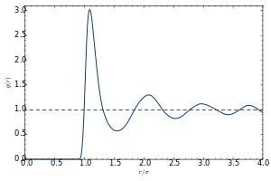

In statistical mechanics, the radial distribution function, (or pair correlation function) in a system of particles (atoms, molecules, colloids, etc.), describes how density varies as a function of distance from a reference particle.
If a given particle is taken to be at the origin O, and if is the average number density of particles, then the local time-averaged density at a distance from O is . This simplified definition holds for a homogeneous and isotropic system. A more general case will be considered below.


In simplest terms it is a measure of the probability of finding a particle at a distance of away from a given reference particle, relative to that for an ideal gas. The general algorithm involves determining how many particles are within a distance of and away from a particle. This general theme is depicted to the right, where the red particle is our reference particle, and blue particles are those which are within the circular shell, dotted in orange.

The RDF is usually determined by calculating the distance between all particle pairs and binning them into a histogram. The histogram is then normalized with respect to an ideal gas, where particle histograms are completely uncorrelated. For three dimensions, this normalization is the number density of the system multiplied by the volume of the spherical shell, which mathematically can be expressed as , where is the number density.


Given a potential energy function, the radial distribution function can be computed either via computer simulation methods like the Monte Carlo method, or via the Ornstein-Zernike equation, using approximative closure relations like the Percus-Yevick approximation or the Hypernetted Chain Theory. It can also be determined experimentally, by radiation scattering techniques or by direct visualization for large enough (micrometer-sized) particles via traditional or confocal microscopy.
The radial distribution function is of fundamental importance since it can be used, using the Kirkwood–Buff solution theory, to link the microscopic details to macroscopic properties. Moreover, by the reversion of the Kirkwood-Buff theory, it is possible to attain the microscopic details of the radial distribution function from the macroscopic properties.
Definition
Consider a system of particles in a volume (for an average number density ) and at a temperature (let us also define ). The particle coordinates are , with . The potential energy due to the interaction between particles is and we do not consider the case of an externally applied field.


The appropriate averages are taken in the canonical ensemble , with the configurational integral, taken over all possible combinations of particle positions. The probability of an elementary configuration, namely finding particle 1 in , particle 2 in , etc. is given by


-
.
(1)

The total number of particles is huge, so that in itself is not very useful. However, one can also obtain the probability of a reduced configuration, where the positions of only particles are fixed, in , with no constraints on the remaining particles. To this end, one has to integrate (1) over the remaining coordinates :


- .

The particles being identical, it is more relevant to consider the probability that any of them occupy positions in any permutation, thus defining the -particle density

-
.
(2)

For , (2) gives the one-particle density which, for a crystal, is a periodic function with sharp maxima at the lattice sites. For a (homogeneous) liquid, it is independent of the position and equal to the overall density of the system:


It is now time to introduce a correlation function by

-
.
(3)

is called a correlation function, since if the atoms are independent from each other would simply equal and therefore corrects for the correlation between atoms.


From (3) and (2) it follows that
-
.
(4)

Relations involving g(r)
The structure factor
The second-order correlation function is of special importance, as it is directly related (via a Fourier transform) to the structure factor of the system and can thus be determined experimentally using X-ray diffraction or neutron diffraction.

If the system consists of spherically symmetric particles, depends only on the relative distance between them, . We will drop the sub- and superscript: . Taking particle 0 as fixed at the origin of the coordinates, is the average number of particles (among the remaining ) to be found in the volume around the position .


We can formally count these particles and take the average via the expression , with the ensemble average, yielding:


-
(5)

where the second equality requires the equivalence of particles . The formula above is useful for relating to the static structure factor , defined by , since we have:


![{\begin{aligned}S(\mathbf {q} )&=1+{\frac {1}{N}}\langle \sum _{i\neq j}\mathrm {e} ^{-i\mathbf {q} (\mathbf {r} _{i}-\mathbf {r} _{j})}\rangle =1+{\frac {1}{N}}\left\langle \int _{V}\mathrm {d} \mathbf {r} \,\mathrm {e} ^{-i\mathbf {q} \mathbf {r} }\sum _{i\neq j}\delta \left[\mathbf {r} -(\mathbf {r} _{i}-\mathbf {r} _{j})\right]\right\rangle \\&=1+{\frac {N(N-1)}{N}}\int _{V}\mathrm {d} \mathbf {r} \,\mathrm {e} ^{-i\mathbf {q} \mathbf {r} }\left\langle \delta (\mathbf {r} -\mathbf {r} _{1})\right\rangle \end{aligned}}](../I/m/6a9027a6f636fa109fcc6bad62b1db5371a05852.svg)
, and thus:
, proving the Fourier relation alluded to above.

This equation is only valid in the sense of distributions, since is not normalized: , so that diverges as the volume , leading to a Dirac peak at the origin for the structure factor. Since this contribution is inaccessible experimentally we can subtract it from the equation above and redefine the structure factor as a regular function:


- .
![S'(\mathbf {q} )=S(\mathbf {q} )-\rho \delta (\mathbf {q} )=1+\rho \int _{V}\mathrm {d} \mathbf {r} \,\mathrm {e} ^{-i\mathbf {q} \mathbf {r} }[g(\mathbf {r} )-1]](../I/m/cf4f160a335264a69b5105ce49e780b1ef411879.svg)
Finally, we rename and, if the system is a liquid, we can invoke its isotropy:

-
.
(6)
![S(q)=1+\rho \int _{V}\mathrm {d} \mathbf {r} \,\mathrm {e} ^{-i\mathbf {q} \mathbf {r} }[g(r)-1]=1+4\pi \rho {\frac {1}{q}}\int \mathrm {d} r\,r\,\mathrm {sin} (qr)[g(r)-1]](../I/m/63765a9a1e6defe6d8aa45956cfb4715b75e64b0.svg)
The compressibility equation
Evaluating (6) in and using the relation between the isothermal compressibility and the structure factor at the origin yields the compressibility equation:


-
.
(7)
![\rho kT\chi _{T}=kT\left({\frac {\partial \rho }{\partial p}}\right)=1+\rho \int _{V}\mathrm {d} \mathbf {r} \,[g(r)-1]](../I/m/a582bdf4e04484354131cd24f5c2fe85b290ca65.svg)
The potential of mean force
It can be shown[1] that the radial distribution function is related to the two-particle potential of mean force by:

-
.
(8)
![g(r)=\exp \left[-{\frac {w^{(2)}(r)}{kT}}\right]](../I/m/531f329551577307c3ddc4aa8055b3c8d4a26941.svg)
The energy equation
If the particles interact via identical pairwise potentials: , the average internal energy per particle is:[2]:Section 2.5

-
.
(9)

The pressure equation of state
Developing the virial equation yields the pressure equation of state:
-
.
(10)

Thermodynamic properties
The radial distribution function is an important measure because several key thermodynamic properties, such as potential energy and pressure can be calculated from it.
For a 3-D system where particles interact via pairwise potentials, the potential energy of the system can be calculated as follows:[3]

Where N is the number of particles in the system, is the number density, is the pair potential.

The pressure of the system can also be calculated by relating the 2nd virial coefficient to . The pressure can be calculated as follows:[3]

Where is the temperature and is Boltzmann's constant. Note that the results of potential and pressure will not be as accurate as directly calculating these properties because of the averaging involved with the calculation of .

Approximations
For dilute systems (e.g. gases), the correlations in the positions of the particles that accounts for are only due to the potential engendered by the reference particle, neglecting indirect effects. In the first approximation, it is thus simply given by the Boltzmann distribution law:
-
.
(11)
![g(r)=\exp \left[-{\frac {u(r)}{kT}}\right]](../I/m/2c8761c3aee52bf4ac06f0d6e81e43a7ab14636b.svg)
If were zero for all – i.e., if the particles did not exert any influence on each other, then for all and the mean local density would be equal to the mean density : the presence of a particle at O would not influence the particle distribution around it and the gas would be ideal. For distances such that is significant, the mean local density will differ from the mean density , depending on the sign of (higher for negative interaction energy and lower for positive ).


As the density of the gas increases, the low-density limit becomes less and less accurate since a particle situated in experiences not only the interaction with the particle in O but also with the other neighbours, themselves influenced by the reference particle. This mediated interaction increases with the density, since there are more neighbours to interact with: it makes physical sense to write a density expansion of , which resembles the virial equation:

-
.
(12)
![g(r)=\exp \left[-{\frac {u(r)}{kT}}\right]y(r)\quad \mathrm {with} \quad y(r)=1+\sum _{n=1}^{\infty }\rho ^{n}y_{n}(r)](../I/m/3da5dfb6e3cbbd32be0d6a4fdcfef111315b3c97.svg)
This similarity is not accidental; indeed, substituting (12) in the relations above for the thermodynamic parameters (Equations 7, 9 and 10) yields the corresponding virial expansions.[4] The auxiliary function is known as the cavity distribution function.[2]:Table 4.1

Experimental
One can determine indirectly (via its relation with the structure factor ) using neutron scattering or x-ray scattering data. The technique can be used at very short length scales (down to the atomic level[5]) but involves significant space and time averaging (over the sample size and the acquisition time, respectively). In this way, the radial distribution function has been determined for a wide variety of systems, ranging from liquid metals[6] to charged colloids.[7] It should be noted that going from the experimental to is not straightforward and the analysis can be quite involved.[8]

It is also possible to calculate directly by extracting particle positions from traditional or confocal microscopy.[9] This technique is limited to particles large enough for optical detection (in the micrometer range), but it has the advantage of being time-resolved so that, aside from the statical information, it also gives access to dynamical parameters (e.g. diffusion constants[10]) and also space-resolved (to the level of the individual particle), allowing it to reveal the morphology and dynamics of local structures in colloidal crystals,[11] glasses,[12] gels,[13][14] and hydrodynamic interactions.[15]
Higher-order correlation functions
Higher-order distribution functions with were less studied, since they are generally less important for the thermodynamics of the system; at the same time, they are not accessible by conventional scattering techniques. They can however be measured by coherent X-ray scattering and are interesting insofar as they can reveal local symmetries in disordered systems.[16]


References
- ↑ Chandler, D. (1987). "7.3". Introduction to Modern Statistical Mechanics. Oxford University Press.
- 1 2 Hansen, J. P. and McDonald, I. R. (2005). Theory of Simple Liquids (3rd ed.). Academic Press.
- 1 2 Frenkel, Daan; Smit, Berend (2002). Understanding molecular simulation from algorithms to applications (2nd ed.). San Diego: Academic Press. ISBN 0122673514.
- ↑ Barker, J.; Henderson, D. (1976). "What is "liquid"? Understanding the states of matter". Reviews of Modern Physics. 48 (4): 587. Bibcode:1976RvMP...48..587B. doi:10.1103/RevModPhys.48.587.
- ↑ Yarnell, J.; Katz, M.; Wenzel, R.; Koenig, S. (1973). "Structure Factor and Radial Distribution Function for Liquid Argon at 85 °K". Physical Review A. 7 (6): 2130. Bibcode:1973PhRvA...7.2130Y. doi:10.1103/PhysRevA.7.2130.
- ↑ Gingrich, N. S.; Heaton, L. (1961). "Structure of Alkali Metals in the Liquid State". The Journal of Chemical Physics. 34 (3): 873. Bibcode:1961JChPh..34..873G. doi:10.1063/1.1731688.
- ↑ Sirota, E.; Ou-Yang, H.; Sinha, S.; Chaikin, P.; Axe, J.; Fujii, Y. (1989). "Complete phase diagram of a charged colloidal system: A synchro- tron x-ray scattering study". Physical Review Letters. 62 (13): 1524–1527. Bibcode:1989PhRvL..62.1524S. doi:10.1103/PhysRevLett.62.1524. PMID 10039696.
- ↑ Pedersen, J. S. (1997). "Analysis of small-angle scattering data from colloids and polymer solutions: Modeling and least-squares fitting". Advances in Colloid and Interface Science. 70: 171–201. doi:10.1016/S0001-8686(97)00312-6.
- ↑ Crocker, J. C.; Grier, D. G. (1996). "Methods of Digital Video Microscopy for Colloidal Studies". Journal of Colloid and Interface Science. 179: 298–201. doi:10.1006/jcis.1996.0217.
- ↑ Nakroshis, P.; Amoroso, M.; Legere, J.; Smith, C. (2003). "Measuring Boltzmann's constant using video microscopy of Brownian motion". American Journal of Physics. 71 (6): 568. Bibcode:2003AmJPh..71..568N. doi:10.1119/1.1542619.
- ↑ Gasser, U.; Weeks, E. R.; Schofield, A.; Pusey, P. N.; Weitz, D. A. (2001). "Real-Space Imaging of Nucleation and Growth in Colloidal Crystallization". Science. 292 (5515): 258–262. Bibcode:2001Sci...292..258G. doi:10.1126/science.1058457. PMID 11303095.
- ↑ Weeks, E. R.; Crocker, J. C.; Levitt, A. C.; Schofield, A.; Weitz, D. A. (2000). "Three-Dimensional Direct Imaging of Structural Relaxation Near the Colloidal Glass Transition". Science. 287 (5453): 627–631. Bibcode:2000Sci...287..627W. doi:10.1126/science.287.5453.627. PMID 10649991.
- ↑ Cipelletti, L.; Manley, S.; Ball, R. C.; Weitz, D. A. (2000). "Universal Aging Features in the Restructuring of Fractal Colloidal Gels". Physical Review Letters. 84 (10): 2275–2278. Bibcode:2000PhRvL..84.2275C. doi:10.1103/PhysRevLett.84.2275. PMID 11017262.
- ↑ Varadan, P.; Solomon, M. J. (2003). "Direct Visualization of Long-Range Heterogeneous Structure in Dense Colloidal Gels". Langmuir. 19 (3): 509. doi:10.1021/la026303j.
- ↑ Gao, C.; Kulkarni, S. D.; Morris, J. F.; Gilchrist, J. F. (2010). "Direct investigation of anisotropic suspension structure in pressure-driven flow". Physical Review E. 81 (4). Bibcode:2010PhRvE..81d1403G. doi:10.1103/PhysRevE.81.041403.
- ↑ Wochner, P.; Gutt, C.; Autenrieth, T.; Demmer, T.; Bugaev, V.; Ortiz, A. D.; Duri, A.; Zontone, F.; Grubel, G.; Dosch, H. (2009). "X-ray cross correlation analysis uncovers hidden local symmetries in disordered matter". Proceedings of the National Academy of Sciences. 106 (28): 11511. Bibcode:2009PNAS..10611511W. doi:10.1073/pnas.0905337106.
- Widom, B. (2002). Statistical Mechanics: A Concise Introduction for Chemists. Cambridge University Press.
- McQuarrie, D. A. (1976). Statistical Mechanics. Harper Collins Publishers.