QUICK scheme
In computational fluid dynamics QUICK, which stands for Quadratic Upstream Interpolation for Convective Kinematics, is a higher-order differencing scheme that considers a three-point upstream weighted quadratic interpolation for the cell phase values. In computational fluid dynamics there are many solution methods for solving the steady convection–diffusion equation. Some of the used methods are the central differencing scheme, upwind scheme, hybrid scheme, power law scheme and QUICK scheme.
The QUICK scheme was presented by Brian P. Leonard – together with the QUICKEST (QUICK with Estimated Streaming Terms) scheme – in a 1979 paper.[1]
In order to find the cell face value a quadratic function passing through two bracketing or surrounding nodes and one node on the upstream side must be used. In central differencing scheme and second order upwind scheme the first order derivative is included and the second order derivative is ignored. These schemes are therefore considered second order accurate where as QUICK does take the second order derivative into account, but ignores the third order derivative hence this is considered third order accurate.[2] This scheme is used to solve convection–diffusion equations using second order central difference for the diffusion term and for the convection term the scheme is third order accurate in space and first order accurate in time. QUICK is most appropriate for steady flow or quasi-steady highly convective elliptic flow.[3]
Quadratic interpolation for QUICK scheme
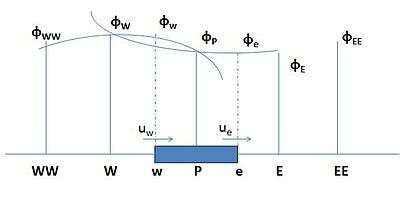
For the one-dimensional domain shown in the figure the Φ value at a control volume face is approximated using three-point quadratic function passing through the two bracketing or surrounding nodes and one other node on upstream side.[4] In the figure, in order to calculate the value of the property at the face, we should have three nodes i.e. two bracketing or surrounding nodes and one upstream node.
- Φw when uw > 0 and ue > 0 a quadratic fit through WW, W and P is used,
- Φe when uw > 0 and ue > 0 a quadratic fit through W, P and E is used,
- Φw when uw < 0 and ue < 0 values of W, P and E are used,
- Φe when uw < 0 and ue < 0 values of P, E and EE are used.
Let the two bracketing nodes be i and i − 1 and upstream node i – 2 then for a uniform grid the value of φ at the cell face between the three nodes is given by:
- Φface = 6⁄8 Φi-1 + 3⁄8 Φi − 1⁄8 Φi-2.
Interpretation of the property when the flow is in different directions
The steady convection and diffusion of a property 'Ƥ' in a given one-dimensional flow field with velocity 'u' and in the absence of sources is given

For the continuity of the flow it must also satisfy

Discretizing the above equation to a control volume around a particular node we get

Integrating this continuity equation over the control volume we get
(ρuA)e - (ρuA)w = 0
now assuming F = ρu and D = r/δx
The corresponding cell face values of the above variables are given by
Fw = (ρu)w
Fe = (ρu)e
Dw = rw /δxWP
De = re /δxPE
Assuming constant area over the entire control volume we get
- FeΦe – FwΦw = De(ΦE – ΦP) – Dw (ΦP - ΦW)
Positive direction
When the flow is in positive direction the values of the velocities will be uw > 0 and ue > 0,
For "w (west face)" bracketing nodes are W and P, the upstream node is WW then,[5]
- Φw = 6/8ΦW + 3/8ΦP − 1/8ΦWW
For "e (east face)" bracketing nodes are P and E, the upstream node is W then
- Φe = 6/8ΦP + 3/8ΦE − 1/8ΦW
Gradient of parabola is used to evaluate diffusion terms.
If Fw > 0 and Fe > 0 and if we use above equations for the convective terms and central differencing for the diffusion terms, the discretized form of the one-dimensional convection–diffusion transport equation will be written as:
- FeΦe – FwΦw = De(ΦE – ΦP) – Dw (ΦP - ΦW)
- Fe(6/8Φp + 3/8ΦE – 1/8Φw) – FW(6/8Φw + 3/8Φp – 1/8Φww) = De(ΦE – ΦP) – DW(Φp – Φw).
On re-arranging we get
- [Dw – 3/8Fw + De + 6/8Fe] ΦP = [Dw + 6/8Fw + 1/8Fe] ΦW + [De – 3/8Fe] ΦE – 1/8FwΦWW,
now it can be written in the standard form:
- aPΦP = aWΦW + aEΦE + aWWΦWW.
where:
| aW | aE | aWW | aP |
|---|---|---|---|
| Dw + 6/8Fw + 1/8Fe | De - 3/8Fe | - 1/8Fw | aw + aE + aWW + (Fe - Fw) |
Negative direction
When the flow is in negative direction the value of the velocities will be uw < 0 and ue < 0,
For west face w the bracketing nodes are W and P, upstream node is E and for the east face E the bracketing nodes are P and E, upstream node is EE
For Fw < 0 and Fe < 0 the flux across the west and east boundaries is given by the expressions :
- Φw = 6/8ΦP + 3/8ΦW - 1/8ΦE
- Φe = 6/8ΦE + 3/8ΦP - 1/8ΦEE
Substitution of these two formulae for the convective terms in the discretized convection-diffusion equation together with central differencing for the diffusion terms leads, after re-arrangement similar to positive direction as above, to the following coefficients.
| aW | aE | aEE | aP |
|---|---|---|---|
| Dw + 3/8Fw | De - 6/8Fe - 1/8Fw | 1/8Fe | aw + aE + aEE + (Fe - Fw) |
QUICK scheme for 1-D convection–diffusion problems
- aPΦP = aWΦW + aEΦE + aWWΦWW + aEEΦEE
Here, aP = aW + aE + aWW + aEE + (Fe - Fw)
other coefficients
| aW | aWW | aE | aEE |
|---|---|---|---|
| Dw + 6/8 αw Fw
+ 1/8Fe αe +3/8 (1 – αw)Fw |
−1/8 αwFw | De - 3/8αe Fe
-6/8(1–αe)Fe −1/8 (1–αw)Fw |
1/8(1 – αe)Fe |
where
- αw=1 for Fw > 0 and αe=1 for Fe > 0
- αw=0 for Fw < 0 and αe=0 for Fe < 0.
Comparing the solutions of QUICK and upwind schemes
From the below graph we can see that the QUICK scheme is more accurate than the upwind scheme. In the QUICK scheme we face the problems of undershoot and overshoot due to which some errors occur. These overshoots and undershoots should be considered while interpreting solutions. False diffusion errors will be minimized with the QUICK scheme when compared with other schemes.

See also
References
- ↑ Leonard, B.P. (1979), "A stable and accurate convective modelling procedure based on quadratic upstream interpolation", Computer Methods in Applied Mechanics and Engineering, 19 (1): 59–98, Bibcode:1979CMAME..19...59L, doi:10.1016/0045-7825(79)90034-3
- ↑ Versteeg, H. K.; Malalasekera, W. (1995), An introduction to computational fluid dynamics, pp. 125–132, ISBN 0-470-23515-2
- ↑ Lin, Pengzhi, Numerical Modeling of Water Waves: An Introduction to Engineers and Scientists, p. 145, ISBN 0-415-41578-0
- ↑ Mitra, Sushanta K.; Chakraborty, Suman, Microfluidics and Nanofluidics Handbook: Fabrication, Implementation, and Applications, p. 161, ISBN 1-4398-1671-9
- ↑ Jakobsen, Hugo A., Chemical Reactor Modeling: Multiphase Reactive Flows, p. 1029, ISBN 3-540-25197-9
Further reading
- Patankar, Suhas V. (1980), Numerical Heat Transfer and Fluid Flow, Taylor & Francis Group, ISBN 978-0-89116-522-4
- Wesseling, Pieter (2001), Principles of Computational Fluid Dynamics, Springer, ISBN 978-3-540-67853-3
- Date, Anil W. (2005), Introduction to Computational Fluid Dynamics, Cambridge University Press, ISBN 978-0-521-85326-2