Pole–zero plot
In mathematics, signal processing and control theory, a pole–zero plot is a graphical representation of a rational transfer function in the complex plane which helps to convey certain properties of the system such as:
- Stability
- Causal system / anticausal system
- Region of convergence (ROC)
- Minimum phase / non minimum phase
A pole-zero plot shows the location in the complex plane of the poles and zeros of the transfer function of a dynamic system, such as a controller, compensator, sensor, equalizer, filter, or communications channel. By convention, the poles of the system are indicated in the plot by an X while the zeroes are indicated by a circle or O.
A pole-zero plot can represent either a continuous-time (CT) or a discrete-time (DT) system. For a CT system, the plane in which the poles and zeros appear is the s plane of the Laplace transform. In this context, the parameter s represents the complex angular frequency, which is the domain of the CT transfer function. For a DT system, the plane is the z plane, where z represents the domain of the Z-transform.
Continuous-time systems
In general, a rational transfer function for a continuous-time LTI system has the form:

where
- and are polynomials in ,
- is the order of the numerator polynomial,
- is the m-th coefficient of the numerator polynomial,
- is the order of the denominator polynomial, and
- is the n-th coefficient of the denominator polynomial.


Either M or N or both may be zero, but in real systems, it should be the case that ; otherwise the gain would be unbounded at high frequencies.

Poles and zeros
- the zeros of the system are roots of the numerator polynomial:
such that


- the poles of the system are roots of the denominator polynomial:
such that .


Region of convergence
The region of convergence (ROC) for a given CT transfer function is a half-plane or vertical strip, either of which contains no poles. In general, the ROC is not unique, and the particular ROC in any given case depends on whether the system is causal or anti-causal.
- If the ROC includes the imaginary axis, then the system is bounded-input, bounded-output (BIBO) stable.
- If the ROC extends rightward from the pole with the largest real-part (but not at infinity), then the system is causal.
- If the ROC extends leftward from the pole with the smallest real-part (but not at negative infinity), then the system is anti-causal.
The ROC is usually chosen to include the imaginary axis since it is important for most practical systems to have BIBO stability.
Example

This system has no (finite) zeros and two poles:

and

The pole-zero plot would be:
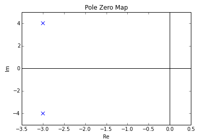
Notice that these two poles are complex conjugates, which is the necessary and sufficient condition to have real-valued coefficients in the differential equation representing the system.
Discrete-time systems
In general, a rational transfer function for a discrete-time LTI system has the form:

where
- is the order of the numerator polynomial,
- is the m-th coefficient of the numerator polynomial,
- is the order of the denominator polynomial, and
- is the n-th coefficient of the denominator polynomial.
Either M or N or both may be zero.
Poles and zeros


Region of convergence
The region of convergence (ROC) for a given DT transfer function is a disk or annulus which contains no poles. In general, the ROC is not unique, and the particular ROC in any given case depends on whether the system is causal or anti-causal.
- If the ROC includes the unit circle, then the system is bounded-input, bounded-output (BIBO) stable.
- If the ROC extends outward from the pole with the largest (but not infinite) magnitude, then the system has a right-sided impulse response. If the ROC extends outward from the pole with the largest magnitude and there is no pole at infinity, then the system is causal.
- If the ROC extends inward from the pole with the smallest (nonzero) magnitude, then the system is anti-causal.
The ROC is usually chosen to include the unit circle since it is important for most practical systems to have BIBO stability.
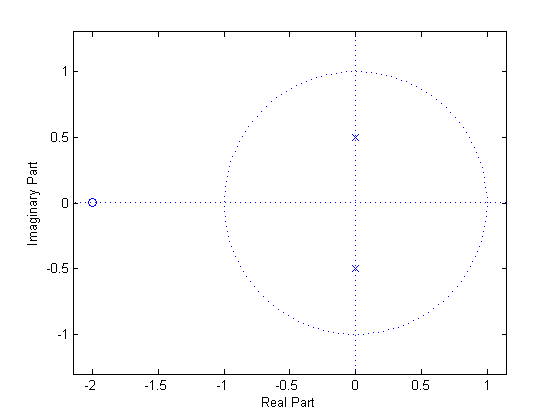
Example
If and are completely factored, their solution can be easily plotted in the z-plane. For example, given the following transfer function:


The only (finite) zero is located at: , and the two poles are located at: , where j is the imaginary unit.


The pole–zero plot would be:
See also
Bibliography
- Haag, Michael (June 22, 2005). "Understanding Pole/Zero Plots on the Z-Plane". Connexions. Retrieved January 24, 2010.
- Eric W. Weisstein. "Z-Transform". MathWorld. Retrieved January 24, 2010.