Pentagram map

In mathematics, the pentagram map is a discrete dynamical system on the moduli space of polygons in the projective plane. The pentagram map takes a given polygon, finds the intersections of the shortest diagonals of the polygon, and constructs a new polygon from these intersections. Richard Schwartz introduced the pentagram map for a general polygon in a 1992 paper ^[1] though it seems that the special case, in which the map is defined for pentagons only, goes back to an 1871 paper of Alfred Clebsch^[2] and a 1945 paper of Theodore Motzkin.^[3] The pentagram map is similar in spirit to the constructions underlying Desargues' Theorem and Poncelet's porism. It echoes the rationale and construction underlying a conjecture of Branko Grünbaum concerning the diagonals of a polygon. ^[4]

Definition of the map

Basic construction

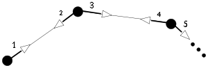
Suppose that the vertices of the polygon P are given by $P_1,P_3,P_5,\ldots$ The image of P under the pentagram map is the polygon Q with vertices $Q_2,Q_4,Q_6,\ldots$ as shown in the figure. Here $Q_4$ is the intersection of the diagonals $(P_1P_5)$ and $(P_3P_7)$ , and so on.

On a basic level, one can think of the pentagram map as an operation defined on convex polygons in the plane. From a more sophisticated point of view, the pentagram map is defined for a polygon contained in the projective plane over a field provided that the vertices are in sufficiently general position. The pentagram map commutes with projective transformations and thereby induces a mapping on the moduli space of projective equivalence classes of polygons.

Labeling conventions

The map $P \to Q$ is slightly problematic, in the sense that the indices of the P-vertices are naturally odd integers whereas the indices of Q-vertices are naturally even integers. A more conventional approach to the labeling would be to label the vertices of P and Q by integers of the same parity. One can arrange this either by adding or subtracting 1 from each of the indices of the Q-vertices. Either choice is equally canonical. An even more conventional choice would be to label the vertices of P and Q by consecutive integers, but again there are 2 natural choices for how to align these labellings: Either $Q_{k}$ is just clockwise from $P_{k}$ or just counterclockwise. In most papers on the subject, some choice is made once and for all at the beginning of the paper and then the formulas are tuned to that choice.

There is a perfectly natural way to label the vertices of the second iterate of the pentagram map by consecutive integers. For this reason, the second iterate of the pentagram map is more naturally considered as an iteration defined on labeled polygons. See the figure.

Twisted polygons

The pentagram map is also defined on the larger space of twisted polygons.^[5]

A twisted N-gon is a bi-infinite sequence of points in the projective plane that is N-periodic modulo a projective transformation That is, some projective transformation M carries $P_{k}$ to $P_{N+k}$ for all k. The map M is called the monodromy of the twisted N-gon. When M is the identity, a twisted N-gon can be interpreted as an ordinary N-gon whose vertices have been listed out repeatedly. Thus, a twisted N-gon is a generalization of an ordinary N-gon.

Two twisted N-gons are equivalent if a projective transformation carries one to the other. The moduli space of twisted N-gons is the set of equivalence classes of twisted N-gons. The space of twisted N-gons contains the space of ordinary N-gons as a sub-variety of co-dimension 8.^[5]^[6]

Elementary properties

Action on pentagons and hexagons

The pentagram map is the identity on the moduli space of pentagons.^[1]^[2]^[3] This is to say that there is always a projective transformation carrying a pentagon to its image under the pentagram map.

The map $T^{2}$ is the identity on the space of labeled hexagons.^[1] Here T is the second iterate of the pentagram map, which acts naturally on labeled hexagons, as described above. This is to say that the hexagons $H$ and $T^2(H)$ are equivalent by a label-preserving projective transformation. More precisely, the hexagons $H'$ and $T(H)$ are projectively equivalent, where $H'$ is the labeled hexagon obtained from $H$ by shifting the labels by 3. ^[1] See the figure. It seems entirely possible that this fact was also known in the 19th century.

The action of the pentagram map on pentagons and hexagons is similar in spirit to classical configuration theorems in projective geometry such as Pascal's theorem, Desargues's theorem and others. ^[7]

Exponential shrinking

The iterates of the pentagram map shrink any convex polygon exponentially fast to a point. ^[1] This is to say that the diameter of the nth iterate of a convex polygon is less than $K a^n$ for constants $K>0$ and $0<a<1$ which depend on the initial polygon. Here we are taking about the geometric action on the polygons themselves, not on the moduli space of projective equivalence classes of polygons.

Motivating discussion

This section is meant to give a non-technical overview for much of the remainder of the article. The context for the pentagram map is projective geometry. Projective geometry is the geometry of our vision. When one looks at the top of a glass, which is a circle, one typically sees an ellipse. When one looks at a rectangular door, one sees a typically non-rectangular quadrilateral. Projective transformations convert between the various shapes one can see when looking at same object from different points of view. This is why it plays such an important role in old topics like perspective drawing and new ones like computer vision. Projective geometry is built around the fact that a straight line looks like a straight line from any perspective. The straight lines are the building blocks for the subject. The pentagram map is defined entirely in terms of points and straight lines. This makes it adapted to projective geometry. If you look at the pentagram map from another point of view (i.e., you tilt the paper on which it is drawn) then you are still looking at the pentagram map. This explains the statement that the pentagram map commutes with projective transformations.

The pentagram map is fruitfully considered as a mapping on the moduli space of polygons. A moduli space is an auxiliary space whose points index other objects. For example, in Euclidean geometry, the sum of the angles of a triangle is always 180 degrees. You can specify a triangle (up to scale) by giving 3 positive numbers, $x,y,z$ such that $x+y+z =180.$ So, each point $(x,y,z)$ , satisfying the constraints just mentioned, indexes a triangle (up to scale). One might say that $(x,y,z)$ are coordinates for the moduli space of scale equivalence classes of triangles. If you want to index all possible quadrilaterals, either up to scale or not, you would need some additional parameters. This would lead to a higher-dimensional moduli space. The moduli space relevant to the pentagram map is the moduli space of projective equivalence classes of polygons. Each point in this space corresponds to a polygon, except that two polygons which are different views of each other are considered the same. Since the pentagram map is adapted to projective geometry, as mentioned above, it induces a mapping on this particular moduli space. That is, given any point in the moduli space, you can apply the pentagram map to the corresponding polygon and see what new point you get.

The reason for considering what the pentagram map does to the moduli space is that it gives more salient features of the map. If you just watch, geometrically, what happens to an individual polygon, say a convex polygon, then repeated application shrinks the polygon to a point.^[1] To see things more clearly, you might dilate the shrinking family of polygons so that they all have, say, the same area. If you do this, then typically you will see that the family of polygons gets long and thin.^[1] Now you can change the aspect ratio so as to try to get yet a better view of these polygons. If you do this process as systematically as possible, you find that you are simply looking at what happens to points in the moduli space. The attempts to zoom in to the picture in the most perceptive possible way lead to the introduction of the moduli space.

To explain how the pentagram map acts on the moduli space, one must say a few words about the torus. One way to roughly define the torus is to say that it is the surface of an idealized donut. Another way is that it is the playing field for the Asteroids video game. Yet another way to describe the torus is to say that it is a computer screen with wrap, both left-to-right and up-to-down. The torus is a classical example of what is known in mathematics as a manifold. This is a space that looks somewhat like ordinary Euclidean space at each point, but somehow is hooked together differently. A sphere is another example of a manifold. This is why it took people so long to figure out that the Earth was not flat; on small scales one cannot easily distinguish a sphere from a plane. So, too, with manifolds like the torus. There are higher-dimensional tori as well. You could imagine playing Asteroids in your room, where you can freely go through the walls and ceiling/floor, popping out on the opposite side.

One can do experiments with the pentagram map, where one looks at how this mapping acts on the moduli space of polygons. One starts with a point and just traces what happens to it as the map is applied over and over again. One sees a surprising thing: These points seem to line up along multi-dimensional tori.^[1] These invisible tori fill up the moduli space somewhat like the way the layers of an onion fill up the onion itself, or how the individual cards in a deck fill up the deck. The technical statement is that the tori make a foliation of the moduli space. The tori have half the dimension of the moduli space. For instance, the moduli space of $7$ -gons is $6$ dimensional and the tori in this case are $3$ dimensional.

The tori are invisible subsets of the moduli space. They are only revealed when one does the pentagram map and watches a point move round and round, filling up one of the tori. Roughly speaking, when dynamical systems have these invariant tori, they are called integrable systems. Most of the results in this article have to do with establishing that the pentagram map is an integrable system, that these tori really exist. The monodromy invariants, discussed below, turn out to be the equations for the tori. The Poisson bracket, discussed below, is a more sophisticated math gadget that sort of encodes the local geometry of the tori. What is nice is that the various objects fit together exactly, and together add up to a proof that this torus motion really exists.

Coordinates for the moduli space

Cross-ratio

When the field underlying all the constructions is F, the affine line is just a copy of F. The affine line is a subset of the projective line. Any finite list of points in the projective line can be moved into the affine line by a suitable projective transformation.

Given the four points $t_1,t_2,t_3,t_4$ in the affine line one defines the (inverse) cross ratio

X=\frac{(t_1 - t_2)(t_3 - t_4)}{(t_1 - t_3)(t_2 - t_4)}.

Most authors consider 1/X to be the cross-ratio, and that is why X is called the inverse cross ratio. The inverse cross ratio is invariant under projective transformations and thus makes sense for points in the projective line. However, the formula above only makes sense for points in the affine line.

In the slightly more general set-up below, the cross ratio makes sense for any four collinear points in projective space One just identifies the line containing the points with the projective line by a suitable projective transformation and then uses the formula above. The result is independent of any choices made in the identification. The inverse cross ratio is used in order to define a coordinate system on the moduli space of polygons, both ordinary and twisted.

The corner coordinates

The corner invariants are basic coordinates on the space of twisted polygons.^[5]^[6]^[8] Suppose that P is a polygon. A flag of P is a pair (p,L), where p is a vertex of P and L is an adjacent line of P. Each vertex of P is involved in 2 flags, and likewise each edge of P is involved in 2 flags. The flags of P are ordered according to the orientation of P, as shown in the figure. In this figure, a flag is represented by a thick arrow. Thus, there are 2N flags associated to an N-gon.

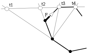
Let P be an N-gon, with flags $F_1,\ldots,F_{2N}$ To each flag F, we associate the inverse cross ratio of the points $t_1,t_2,t_3,t_4$ shown in the figure at left. In this way, one associates numbers $x_1,\ldots,x_{2n}$ to an n-gon. If two n-gons are related by a projective transformation, they get the same coordinates. Sometimes the variables $x_1,y_1,x_2,y_2,\ldots$ are used in place of $x_1,x_2,x_3,x_4,\ldots\,.$

The corner invariants make sense on the moduli space of twisted polygons. When one defines the corner invariants of a twisted polygon, one obtains a 2N-periodic bi-infinite sequence of numbers. Taking one period of this sequence identifies a twisted N-gon with a point in $F^{2N}$ where F is the underlying field. Conversely, given almost any (in the sense of measure theory) point in $F^{2N}$ one can construct a twisted N-gon having this list of corner invariants. Such a list will not always give rise to an ordinary polygon; there are an additional 8 equations which the list must satisfy for it to give rise to an ordinary N-gon.

(ab) coordinates

There is a second set of coordinates for the moduli space of twisted polygons, developed by Sergei Tabachnikov and Valentin Ovsienko. ^[6] One describes a polygon in the projective plane by a sequence of vectors $\ldots V_1,V_2,V_3,\ldots$ in $R^3$ so that each consecutive triple of vectors spans a parallelopiped having unit volume. This leads to the relation

$V_{i+3} = a_i V_{i+2} + b_i V_{i+1} + V_i$

The coordinates $a_1,b_1,a_2,b_2,\ldots$ serve as coordinates for the moduli space of twisted N-gons as long as N is not divisible by 3.

The (ab) coordinates bring out the close analogy between twisted polygons and solutions of 3rd order linear ordinary differential equations, normalized to have unit Wronskian.

Formula for the pentagram map

As a birational mapping

Here is a formula for the pentagram map, expressed in corner coordinates.^[5] The equations work more gracefully when one considers the second iterate of the pentagram map, thanks to the canonical labelling scheme discussed above. The second iterate of the pentagram map is the composition $B \circ A$ . The maps $A$ and $B$ are birational mappings of order 2, and have the following action.

$A(x_1,\ldots,x_{2N})=(a_1,\ldots,a_{2N})$
$B(x_1,\ldots,x_{2N})=(b_1,\ldots,b_{2N})$

where

$a_{2k-1}=\frac{(1-x_{2k+1}x_{2k+2})}{(1-x_{2k-3}x_{2k-2})} x_{2k+0}$
$a_{2k+0}=\frac{(1-x_{2k-3}x_{2k-2})}{(1-x_{2k+1}x_{2k+2})} x_{2k-1}$
$b_{2k+1}=\frac{(1-x_{2k-2}x_{2k-1})}{(1-x_{2k+2}x_{2k+3})} x_{2k+0}$
$b_{2k+0}=\frac{(1-x_{2k+2}x_{2k+3})}{(1-x_{2k-2}x_{2k-1})} x_{2k-1}$

(Note: the index 2k+0 is just 2k. The 0 is added to align the formulas.) In these coordinates, the pentagram map is a birational mapping of $F^{2N}$

As grid compatibility relations

The formula for the pentagram map has a convenient interpretation as a certain compatibility rule for labelings on the edges of triangular grid, as shown in the figure.^[5] In this interpretation, the corner invariants of a polygon P label the non-horizontal edges of a single row, and then the non-horizontal edges of subsequent rows are labeled by the corner invariants of $A(P)$ , $B(A(P))$ , $A(B(A(P)))$ , and so forth. the compatibility rules are

c=1-ab
wx=yz

These rules are meant to hold for all configurations which are congruent to the ones shown in the figure. In other words, the figures involved in the relations can be in all possible positions and orientations. The labels on the horizontal edges are simply auxiliary variables introduced to make the formulas simpler. Once a single row of non-horizontal edges is provided, the remaining rows are uniquely determined by the compatibility rules.

Invariant structures

Corner coordinate products

It follows directly from the formula for the pentagram map, in terms of corner coordinates, that the two quantities

$O_N= x_1x_3\cdots x_{2N-1}$
$E_N = x_2x_4\cdots x_{2N}$

are invariant under the pentagram map. This observation is closely related to the 1991 paper of Joseph Zaks ^[4] concerning the diagonals of a polygon.

When N = 2k is even, the functions

$O_k = x_1x_5x_9 \cdots x_{2N-3}+ x_3x_7x_{11} \cdots x_{2N-1}$
$E_k = x_2x_6x_{10} \cdots x_{2N-2}+ x_4x_8x_{12} \cdots x_{2N}$

are likewise seen, directly from the formula, to be invariant functions. All these products turn out to be Casimir invariants with respect to the invariant Poisson bracket discussed below. At the same time, the functions $O_k$ and $E_k$ are the simplest examples of the monodromy invariants defined below.

The level sets of the function $f=O_NE_N$ are compact, when f is restricted to the moduli space of real convex polygons. ^[1] Hence, each orbit of the pentagram map acting on this space has a compact closure.

Volume form

The pentagram map, when acting on the moduli space X of convex polygons, has an invariant volume form. ^[9] At the same time, as was already mentioned, the function $f=O_NE_N$ has compact level sets on X. These two properties combine with the Poincaré recurrence theorem to imply that the action of the pentagram map on X is recurrent: The orbit of almost any equivalence class of convex polygon P returns infinitely often to every neighborhood of P.^[9] This is to say that, modulo projective transformations, one typically sees nearly the same shape, over and over again, as one iterates the pentagram map. (It is important to remember that one is considering the projective equivalence classes of convex polygons. The fact that the pentagram map visibly shrinks a convex polygon is irrelevant.)

It is worth mentioning that the recurrence result is subsumed by the complete integrability results discussed below.^[6]^[10]

Monodromy invariants

The so-called monodromy invariants are a collection of functions on the moduli space that are invariant under the pentagram map. ^[5]

With a view towards defining the monodromy invariants, say that a block is either a single integer or a triple of consecutive integers, for instance 1 and 567. Say that a block is odd if it starts with an odd integer. Say that two blocks are well-separated if they have at least 3 integers between them. For instance 123 and 567 are not well separated but 123 and 789 are well separated. Say that an odd admissible sequence is a finite sequence of integers that decomposes into well separated odd blocks. When we take these sequences from the set 1, ..., 2N, the notion of well separation is meant in the cyclic sense. Thus, 1 and 2N-1 are not well separated.

Each odd admissible sequence gives rise to a monomial in the corner invariants. This is best illustrated by example

1567 gives rise to $- x_1x_5x_6x_7$
123789 gives rise to $+ x_1x_2x_3x_7x_8x_9$

The sign is determined by the parity of the number of single-digit blocks in the sequence. The monodromy invariant $O_k$ is defined as the sum of all monomials coming from odd admissible sequences composed of k blocks. The monodromy invariant $E_k$ is defined the same way, with even replacing odd in the definition.

When N is odd, the allowable values of k are 1, 2, ..., (n − 1)/2. When N is even, the allowable values of k are 1, 2, ..., n/2. When k = n/2, one recovers the product invariants discussed above. In both cases, the invariants $O_N$ and $E_N$ are counted as monodromy invariants, even though they are not produced by the above construction.

The monodromy invariants are defined on the space of twisted polygons, and restrict to give invariants on the space of closed polygons. They have the following geometric interpretation. The monodromy M of a twisted polygon is a certain rational function in the corner coordinates. The monodromy invariants are essentially the homogeneous parts of the trace of M. There is also a description of the monodromy invariants in terms of the (ab) coordinates. In these coordinates, the invariants arise as certain determinants of 4-diagonal matrices. ^[6]^[8]

Whenever P has all its vertices on a conic section (such as a circle) one has $O_k(P)=E_k(P)$ for all k. ^[8]

Poisson bracket

A Poisson bracket is an anti-symmetric linear operator $\{\cdot,\cdot\}$ on the space of functions which satisfies the Leibniz Identity and the Jacobi identity. In a 2010 paper,^[6] Valentin Ovsienko, Richard Schwartz and Sergei Tabachnikov produced a Poisson bracket on the space of twisted polygons which is invariant under the pentagram map. They also showed that monodromy invariants commute with respect to this bracket. This is to say that

$\{O_i,O_j\}=\{O_i,E_j\}=\{E_i,E_j\}=0$

for all indices.

Here is a description of the invariant Poisson bracket in terms of the variables.

x_1,y_1,x_2,y_2,\ldots\,.

\{x_i,x_{i+1}\} = -x_i\, x_{i+1}

\{x_i, x_{i-1}\} = x_i\, x_{i-1}

\{y_i,y_{i+1}\} = y_i\, y_{i+1}

\{y_i,y_{i-1}\} = -y_i\, y_{i-1}

\{x_i,x_j\} = \{y_i,y_j\} = \{x_i,y_j\} = 0

for all other

i,j.

There is also a description in terms of the (ab) coordinates, but it is more complicated.^[6]

Here is an alternate description of the invariant bracket. Given any function $f$ on the moduli space, we have the so-called Hamiltonian vector field

$H(f)=(x_{i+1} \partial f/\partial x_{i+1} - x_{i-1} \partial f/\partial x_{i-1})x_i \partial/\partial x_i + (y_{i-1} \partial f/\partial y_{i-1} - y_{i+1} \partial f/\partial y_{i+1}) y_i \partial/\partial y_i$

where a summation over the repeated indices is understood. Then

$H(f) g = \{f,g\}$

The first expression is the directional derivative of $g$ in the direction of the vector field $H(f)$ . In practical terms, the fact that the monodromy invariants Poisson-commute means that the corresponding Hamiltonian vector fields define commuting flows.

Complete integrability

Arnold–Liouville integrability

The monodromy invariants and the invariant bracket combine to establish Arnold–Liouville integrability of the pentagram map on the space of twisted N-gons. ^[6] The situation is easier to describe for N odd. In this case, the two products

$O_n =x_1\cdots x_n$
$E_n = y_1\cdots y_n$

are Casimir invariants for the bracket, meaning (in this context) that

$\{O_n,f\}=\{E_n,f\} =0$

for all functions f. A Casimir level set is the set of all points in the space having a specified value for both $O_n$ and $E_n$ .

Each Casimir level set has an iso-monodromy foliation, namely, a decomposition into the common level sets of the remaining monodromy functions. The Hamiltonian vector fields associated to the remaining monodromy invariants generically span the tangent distribution to the iso-monodromy foliation. The fact that the monodromy invariants Poisson-commute means that these vector fields define commuting flows. These flows in turn define local coordinate charts on each iso-monodromy level such that the transition maps are Euclidean translations. That is, the Hamiltonian vector fields impart a flat Euclidean structure on the iso-monodromy levels, forcing them to be flat tori when they are smooth and compact manifolds. This happens for almost every level set. Since everything in sight is pentagram-invariant, the pentagram map, restricted to an iso-monodromy leaf, must be a translation. This kind of motion is known as quasi-periodic motion. This explains the Arnold-Liouville integrability.

From the point of view of symplectic geometry, the Poisson bracket gives rise to a symplectic form on each Casimir level set.

Algebro-geometric integrability

In a 2011 preprint, ^[10] Fedor Soloviev showed that the pentagram map has a Lax representation with a spectral parameter, and proved its algebraic-geometric integrability. This means that the space of polygons (either twisted or ordinary) is parametrized in terms of a spectral curve with marked points and a divisor. The spectral curve is determined by the monodromy invariants, and the divisor corresponds to a point on a torus—the Jacobi variety of the spectral curve. The algebraic-geometric methods guarantee that the pentagram map exhibits quasi-periodic motion on a torus (both in the twisted and the ordinary case), and they allow one to construct explicit solutions formulas using Riemann theta functions (i.e., the variables that determine the polygon as explicit functions of time). Soloviev also obtains the invariant Poisson bracket from the Krichever-Phong universal formula.

Connections to other topics

The Octahedral recurrence

The octahedral recurrence is a dynamical system defined on the vertices of the octahedral tiling of space. Each octahedron has 6 vertices, and these vertices are labelled in such a way that

$a_1b_1 + a_2b_2 = a_3b_3$

Here $a_i$ and $b_i$ are the labels of antipodal vertices. A common convention is that $a_2,b_2,a_3,b_3$ always lie in a central horizontal plane and a_1,b_1 are the top and bottom vertices. The octahedral recurrence is closely related to C. L. Dodgson's method of condensation for computing determinants.^[5] Typically one labels two horizontal layers of the tiling and then uses the basic rule to let the labels propagate dynamically.

Max Glick used the cluster algebra formalism to find formulas for the iterates of the pentagram map in terms of alternating sign matrices.^[11] These formulas are similar in spirit to the formulas found by David P. Robbins and Harold Rumsey for the iterates of the octahedral recurrence.

Alternatively, the following construction relates the octahedral recurrence directly to the pentagram map. ^[5] Let $T$ be the octahedral tiling. Let $\pi: T \to R^2$ be the linear projection which maps each octahedron in $T$ to the configuration of 6 points shown in the first figure. Say that an adapted labeling of $T$ is a labeling so that all points in the (infinite) inverse image of any point in $G=\pi(T)$ get the same numerical label. The octahedral recurrence applied to an adapted labeling is the same as a recurrence on $G$ in which the same rule as for the octahedral recurrence is applied to every configuration of points congruent to the configuration in the first figure. Call this the planar octahedral recurrence.

Given a labeling of $G$ which obeys the planar octahedral recurrence, one can create a labeling of the edges of $G$ by applying the rule

$v=AD/BC$

to every edge. This rule refers to the figure at right and is meant to apply to every configuration that is congruent to the two shown.

When this labeling is done, the edge-labeling of G satisfies the relations for the pentagram map.

The Boussinesq equation

The continuous limit of a convex polygon is a parametrized convex curve in the plane. When the time parameter is suitably chosen, the continuous limit of the pentagram map is the classical Boussinesq equation.^[5]^[6] This equation is a classical example of an integrable partial differential equation.

Here is a description of the geometric action of the Boussinesq equation. Given a locally convex curve $C:R->R^2$ , and real numbers x and t, we consider the chord connecting $C(x-t)$ to $C(x+t)$ . The envelop of all these chords is a new curve $C_t(x)$ . When t is extremely small, the curve $C_t(x)$ is a good model for the time t evolution of the original curve $C_0(x)$ under the Boussinesq equation. This geometric description makes it fairly obvious that the B-equation is the continuous limit of the pentagram map. At the same time, the pentagram invariant bracket is a discretization of a well known invariant Poisson bracket associated to the Boussinesq equation. ^[6]

Recently, there has been some work on higher-dimensional generalizations of the pentagram map and its connections to Boussinesq-type partial differential equations ^[12]

Projectively natural evolution

The pentagram map and the Boussinesq equation are examples of projectively natural geometric evolution equations. Such equations arise in diverse fields of mathematics, such as projective geometry and computer vision. ^[13] ^[14]

Cluster algebras

In a 2010 paper ^[11] Max Glick identified the pentagram map as a special case of a cluster algebra.

Notes

1 2 3 4 5 6 7 8 9 Schwartz, Richard Evan (1992). "The Pentagram Map". Journal of Experimental Math. 1: 90–95.
1 2 A. Clebsch (1871). "Ueber das ebene Funfeck". Mathematische Annalen. 4: 476–489. doi:10.1007/bf01455078.
1 2 Th. Motzkin (1945). "The pentagon in the projective plane, with a comment on Napier's rule". Bulletin of the American Mathematical Society. 51 (12): 985–989. doi:10.1090/S0002-9904-1945-08488-2.
1 2 Zaks, Joseph. "On the products of cross-ratios on diagonals of polygons". Geometriae Dedicata. 60 (2): 145–151. doi:10.1007/BF00160619. Retrieved 2010-02-12.
1 2 3 4 5 6 7 8 9 Schwartz, Richard Evan. "Discrete monodromy, pentagrams, and the method of condensation". journal of Fixed Point Theory and Applications (2008). Retrieved 2010-02-12.
1 2 3 4 5 6 7 8 9 10 Ovsienko, Valentin; Schwartz, Richard Evan; Tabachnikov, Serge (2010). "The Pentagram Map, A Discrete Integrable System" (pdf). Comm. Math. Phys. 299 (2): 409–446. Retrieved June 26, 2011.
↑ Schwartz, Richard Evan; Tabachnikov, Serge (October 2009). "Elementary Surprises in Projective Geometry". arXiv:0910.1952.
1 2 3 Schwartz, Richard Evan; Tabachnikov, Sergei (October 2009). "The pentagram integrals for inscribed polygons". Electronic Journal of Combinatorics. arXiv:1004.4311.
1 2 Schwartz, Richard Evan (2001). "Recurrence of the Pentagram Map" (pdf). Journal of Experimental Math. 10 (4): 519–528. doi:10.1080/10586458.2001.10504671. Retrieved June 30, 2011.
1 2 Soloviev, Fedor (2011). "Integrability of the Pentagram Map". arXiv:1106.3950.
1 2
- Glick, Max (2010). "The Pentagram Map and Y-Patterns". arXiv:1005.0598v2.
↑ Beffa, Gloria Marỉ. "On Generalizations of the Pentagram Map: Discretizal of AGD Flows" (pdf). Madison, Wisconsin: University of Wisconsin.
↑ Bruckstein, Alfred M.; Shaked, Doron. "On Projective Invariant Smoothing and Evolutions of Planar Curves and Polygons" (pdf). Journal of Mathematical Imaging and Vision. 7 (3): 225–240. doi:10.1023/A:1008226427785. Retrieved 2010-02-12.
↑ Peter J. Olver; Guillermo Sapiro; Allen Tannenbaum; MINNESOTA UNIV MINNEAPOLIS DEPT OF MATHEMATICS. "Differential Invariant Signatures and Flows in Computer Vision: A Symmetry Group Approach". Retrieved 2010-02-12.

References

Beffa, Gloria Marỉ. "On Generalizations of the Pentagram Map: Discretizal of AGD Flows" (pdf). Madison, Wisconsin: University of Wisconsin.
Bruckstein, Alfred M.; Shaked, Doron. "On Projective Invariant Smoothing and Evolutions of Planar Curves and Polygons" (pdf). Journal of Mathematical Imaging and Vision. 7 (3): 225–240. doi:10.1023/A:1008226427785. Retrieved 2010-02-12.
Glick, Max (2010). "The Pentagram Map and Y-Patterns". arXiv:1005.0598v2.
Motzkin, Theodore (1945). "The pentagon in the projective plane, with a comment on Napier's rule". Bull. Amer. Math. Soc. 51 (12): 985–989. doi:10.1090/S0002-9904-1945-08488-2.
Olver, Peter J.; Sapiro, Guillermo; Tannenbaum, Allen (1993). "Differential Invariant Signatures and Flows in Computer Vision: A Symmetry Group Approach". Minnesota University Minneapolis Department of Mathematics. Retrieved 2010-02-12.
Ovsienko, Valentin; Tabachnikov, Serge. "Discrete integrable systems in projective geometry" (PDF). Retrieved 2010-02-12.
Ovsienko, Valentin; Schwartz, Richard Evan; Tabachnikov, Serge (2010). "The Pentagram Map, A Discrete Integrable System" (pdf). Comm. Math. Phys. 299 (2): 409–446. Retrieved June 26, 2011.
Ovsienko, Valentin; Schwartz, Richard Evan; Tabachnikov, Serge (2009). "Quasiperiodic Motion for the Pentagram Map" (pdf). Electron. Res. Announc. Math. Sci. 16: 1–8. doi:10.3934/era.2009.16.1.
Schwartz, Richard Evan (1992). "The Pentagram Map". Journal of Experimental Math. 1: 90–95.
Schwartz, Richard Evan (2001). "Recurrence of the Pentagram Map" (pdf). Journal of Experimental Math. 10 (4): 519–528. doi:10.1080/10586458.2001.10504671. Retrieved June 30, 2011.
Schwartz, Richard Evan (2008). "Discrete monodromy, pentagrams, and the method of condensation". Journal of Fixed Point Theory and Applications. Retrieved 2010-02-12.
Schwartz, Richard Evan; Tabachnikov, Serge. "The pentagram integrals for inscribed polygons". Electronic Journal of Combinatorics. arXiv:1004.4311.
Schwartz, Richard Evan; Tabachnikov, Serge (2009). "Elementary Surprises in Projective Geometry". arXiv:0910.1952.
Soloviev, Fedor (2011). "Integrability of the Pentagram Map". arXiv:1106.3950.
Zaks, Joseph. "On the products of cross-ratios on diagonals of polygons". Geometriae Dedicata. 60 (2): 145–151. doi:10.1007/BF00160619. Retrieved 2010-02-12.

This article is issued from Wikipedia - version of the 8/19/2016. The text is available under the Creative Commons Attribution/Share Alike but additional terms may apply for the media files.