Nyquist frequency
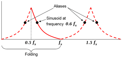
The Nyquist frequency, named after electronic engineer Harry Nyquist, is half of the sampling rate of a discrete signal processing system.[1][2] It is sometimes known as the folding frequency of a sampling system.[3] An example of folding is depicted in Figure 1, where fs is the sampling rate and 0.5 fs is the corresponding Nyquist frequency.[note 1] The black dot plotted at 0.6 fs represents the amplitude and frequency of a sinusoidal function whose frequency is 60% of the sample-rate (fs). The other three dots indicate the frequencies and amplitudes of three other sinusoids that would produce the same set of samples as the actual sinusoid that was sampled. The symmetry about 0.5 fs is referred to as folding.
The Nyquist frequency should not be confused with the Nyquist rate, which is the minimum sampling rate that satisfies the Nyquist sampling criterion for a given signal or family of signals. The Nyquist rate is twice the maximum component frequency of the function being sampled. For example, the Nyquist rate for the sinusoid at 0.6 fs is 1.2 fs, which means that at the fs rate, it is being undersampled. Thus, Nyquist rate is a property of a continuous-time signal, whereas Nyquist frequency is a property of a discrete-time system.[4][5]
When the function domain is time, sample rates are usually expressed in samples/second, and the unit of Nyquist frequency is cycles/second (hertz). When the function domain is distance, as in an image sampling system, the sample rate might be dots per inch and the corresponding Nyquist frequency would be in cycles/inch.
Aliasing
Referring again to Figure 1, undersampling of the sinusoid at 0.6 fs is what allows there to be a lower-frequency alias, which is a different function that produces the same set of samples. That condition is usually described as aliasing. The mathematical algorithms that are typically used to recreate a continuous function from its samples will misinterpret the contributions of undersampled frequency components, which causes distortion. Samples of a pure 0.6 fs sinusoid would produce a 0.4 fs sinusoid instead. If the true frequency was 0.4 fs, there would still be aliases at 0.6, 1.4, 1.6, etc.,[note 2] but the reconstructed frequency would be correct.
In a typical application of sampling, one first chooses the highest frequency to be preserved and recreated, based on the expected content (voice, music, etc.) and desired fidelity. Then one inserts an anti-aliasing filter ahead of the sampler. Its job is to attenuate the frequencies above that limit. Finally, based on the characteristics of the filter, one chooses a sample-rate (and corresponding Nyquist frequency) that will provide an acceptably small amount of aliasing.
In applications where the sample-rate is pre-determined, the filter is chosen based on the Nyquist frequency, rather than vice versa. For example, audio CDs have a sampling rate of 44100 samples/sec. The Nyquist frequency is therefore 22050 Hz. The anti-aliasing filter must adequately suppress any higher frequencies but negligibly affect the frequencies within the human hearing range. A filter that preserves 0–20 kHz is more than adequate for that.
Other meanings
Early uses of the term Nyquist frequency, such as those cited above, are all consistent with the definition presented in this article. Some later publications, including some respectable textbooks, call twice the signal bandwidth the Nyquist frequency;[6][7] this is a distinctly minority usage, and the frequency at twice the signal bandwidth is otherwise commonly referred to as the Nyquist rate.
See also
- Aliasing (a.k.a. folding)
- Kell factor
- Sampling frequency
- Superoscillation
- Signal
Notes
- ↑ In this context, the factor of ½ has units of cycles per sample, as explained at Aliasing#Sampling sinusoidal functions.
- ↑ As previously mentioned, these are the frequencies of other sinusoids that would produce the same set of samples as the one that was actually sampled.
Citations
- ↑ Grenander, Ulf (1959). Probability and Statistics: The Harald Cramér Volume. Wiley.
The Nyquist frequency is that frequency whose period is two sampling intervals.
- ↑ Harry L. Stiltz (1961). Aerospace Telemetry. Prentice-Hall.
the existence of power in the continuous signal spectrum at frequencies higher than the Nyquist frequency is the cause of aliasing error
- ↑ Thomas Zawistowski; Paras Shah. "An Introduction to Sampling Theory". Retrieved 17 April 2010.
Frequencies "fold" around half the sampling frequency - which is why [the Nyquist] frequency is often referred to as the folding frequency.
- ↑ James J. Condon & Scott M. Ransom (2016). Essential Radio Astronomy. Princeton University Press. pp. 280–281. ISBN 9781400881161.
- ↑ John W. Leis (2011). Digital Signal Processing Using MATLAB for Students and Researchers. John Wiley & Sons. p. 82. ISBN 9781118033807.
The Nyquist rate is twice the bandwidth of the signal ... The Nyquist frequency or folding frequency is half the sampling rate and corresponds to the highest frequency which a sampled data system can reproduce without error.
- ↑ Jonathan M. Blackledge (2003). Digital Signal Processing: Mathematical and Computational Methods, Software Development and Applications. Horwood Publishing. ISBN 1-898563-48-9.
- ↑ Paulo Sergio Ramirez Diniz, Eduardo A. B. Da Silva, Sergio L. Netto (2002). Digital Signal Processing: System Analysis and Design. Cambridge University Press. ISBN 0-521-78175-2.