Neutrino oscillation
| Beyond the Standard Model |
|---|
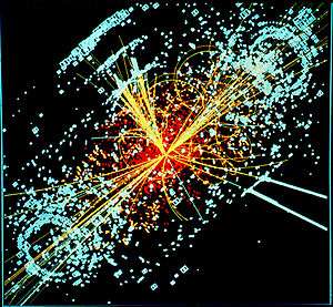 Simulated Large Hadron Collider CMS particle detector data depicting a Higgs boson produced by colliding protons decaying into hadron jets and electrons |
| Standard Model |
Neutrino oscillation is a quantum mechanical phenomenon whereby a neutrino created with a specific lepton flavor (electron, muon, or tau) can later be measured to have a different flavor. The probability of measuring a particular flavor for a neutrino varies periodically as it propagates through space.[1]
First predicted by Bruno Pontecorvo in 1957,[2][3] neutrino oscillation has since been observed by a multitude of experiments in several different contexts. Notably, the existence of neutrino oscillation resolved the long-standing solar neutrino problem.
Neutrino oscillation is of great theoretical and experimental interest, as the precise properties of the process can shed light on several properties of the neutrino. In particular, it implies that the neutrino has a non-zero mass, which requires a modification to the Standard Model of particle physics.[1] The experimental discovery of neutrino oscillation, and thus neutrino mass, by the Super-Kamiokande Observatory and the Sudbury Neutrino Observatories was recognized with the 2015 Nobel Prize for Physics.[4]
Observations
A great deal of evidence for neutrino oscillation has been collected from many sources, over a wide range of neutrino energies and with many different detector technologies.[5] The 2015 Nobel Prize in Physics was shared by Takaaki Kajita and Arthur B. McDonald for their early pioneering observations of these oscillations.
Neutrino oscillation is a function of the ratio L/E, where is L the distance traveled and E is the neutrino's energy. (Details in § Propagation and interference below.) Neutrino sources and detectors are far too large to move, but all available sources produce a range of energies, and oscillation can be measured with a fixed distance and neutrinos of varying energy. The preferred distance depends on the most common energy, but the exact distance is not critical as long as it is known. The limiting factor in measurements is the accuracy with which the energy of each observed neutrino can be measured. Because current detectors have energy uncertainties of a few percent, it is satisfactory to know the distance to within 1%.
Solar neutrino oscillation
The first experiment that detected the effects of neutrino oscillation was Ray Davis's Homestake Experiment in the late 1960s, in which he observed a deficit in the flux of solar neutrinos with respect to the prediction of the Standard Solar Model, using a chlorine-based detector.[6] This gave rise to the Solar neutrino problem. Many subsequent radiochemical and water Cherenkov detectors confirmed the deficit, but neutrino oscillation was not conclusively identified as the source of the deficit until the Sudbury Neutrino Observatory provided clear evidence of neutrino flavor change in 2001.[7]
Solar neutrinos have energies below 20 MeV. At energies above 5 MeV, solar neutrino oscillation actually takes place in the Sun through a resonance known as the MSW effect, a different process from the vacuum oscillation described later in this article.[1]
Atmospheric neutrino oscillation
Large detectors such as IMB, MACRO, and Kamiokande II have observed a deficit in the ratio of the flux of muon to electron flavor atmospheric neutrinos (see muon decay). The Super-Kamiokande experiment provided a very precise measurement of neutrino oscillation in an energy range of hundreds of MeV to a few TeV, and with a baseline of the diameter of the Earth; the first experimental evidence for atmospheric neutrino oscillations was announced in 1998.[8]
Reactor neutrino oscillation
Many experiments have searched for oscillation of electron anti-neutrinos produced at nuclear reactors. Such oscillations give the value of the parameter θ13. Neutrinos produced in nuclear reactors have energies similar to solar neutrinos, of around a few MeV. The baselines of these experiments have ranged from tens of meters to over 100 km.
In 2012, the Daya Bay experiment announced a discovery that θ13 ≠ 0 with a significance of 5.2σ;[9] these results have since been confirmed by RENO[10] and Double Chooz.
Beam neutrino oscillation
Neutrino beams produced at a particle accelerator offer the greatest control over the neutrinos being studied. Many experiments have taken place that study the same oscillations as in atmospheric neutrino oscillation using neutrinos with a few GeV of energy and several-hundred-km baselines. The MINOS, K2K, and Super-K experiments have all independently observed muon neutrino disappearance over such long baselines.[1]
Data from the LSND experiment appear to be in conflict with the oscillation parameters measured in other experiments. Results from the MiniBooNE appeared in Spring 2007 and contradicted the results from LSND, although they could support the existence of a fourth neutrino type, the sterile neutrino.[1]
In 2010, the INFN and CERN announced the observation of a tau particle in a muon neutrino beam in the OPERA detector located at Gran Sasso, 730 km away from the source in Geneva.[11]
T2K, using a neutrino beam directed through 295 km of earth and the Super-Kamiokande detector, measured a non-zero value for the parameter θ13 in a neutrino beam.[12] NOνA, using the same beam as MINOS with a baseline of 810 km, is sensitive to the same.
Theory
Neutrino oscillation arises from a mixture between the flavor and mass eigenstates of neutrinos. That is, the three neutrino states that interact with the charged leptons in weak interactions are each a different superposition of the three neutrino states of definite mass. Neutrinos are created in weak processes in their flavor eigenstates[nb 1]. As a neutrino propagates through space, the quantum mechanical phases of the three mass states advance at slightly different rates due to the slight differences in the neutrino masses. This results in a changing mixture of mass states as the neutrino travels, but a different mixture of mass states corresponds to a different mixture of flavor states. So a neutrino born as, say, an electron neutrino will be some mixture of electron, mu, and tau neutrino after traveling some distance. Since the quantum mechanical phase advances in a periodic fashion, after some distance the state will nearly return to the original mixture, and the neutrino will be again mostly electron neutrino. The electron flavor content of the neutrino will then continue to oscillate as long as the quantum mechanical state maintains coherence. Since mass differences between neutrino flavors are small in comparison with long coherence length for neutrino oscillations this microscopic quantum effect becomes observable over macroscopic distances.
Pontecorvo–Maki–Nakagawa–Sakata matrix
The idea of neutrino oscillation was first put forward in 1957 by Bruno Pontecorvo, who proposed that neutrino-antineutrino transitions may occur in analogy with neutral kaon mixing.[2] Although such matter-antimatter oscillation has not been observed, this idea formed the conceptual foundation for the quantitative theory of neutrino flavor oscillation, which was first developed by Maki, Nakagawa, and Sakata in 1962[14] and further elaborated by Pontecorvo in 1967.[3] One year later the solar neutrino deficit was first observed,[15] and that was followed by the famous paper of Gribov and Pontecorvo published in 1969 titled "Neutrino astronomy and lepton charge".[16]
The concept of neutrino mixing is a natural outcome of gauge theories with massive neutrinos and its structure can be characterized in general.[17] In its simplest form it is expressed as a unitary transformation relating the flavor and mass eigenbasis, and can be written


where
- is a neutrino with definite flavor. α = e (electron), μ (muon) or τ (tauon).
- is a neutrino with definite mass , 1, 2, 3.
- The asterisk () represents a complex conjugate. For antineutrinos, the complex conjugate should be dropped from the first equation, and added to the second.


represents the Pontecorvo–Maki–Nakagawa–Sakata matrix (also called the PMNS matrix, lepton mixing matrix, or sometimes simply the MNS matrix). It is the analogue of the CKM matrix describing the analogous mixing of quarks. If this matrix were the identity matrix, then the flavor eigenstates would be the same as the mass eigenstates. However, experiment shows that it is not.

When the standard three neutrino theory is considered, the matrix is 3×3. If only two neutrinos are considered, a 2×2 matrix is used. If one or more sterile neutrinos are added (see later) it is 4×4 or larger. In the 3×3 form, it is given by:[18]

where cij = cos θij and sij = sin θij. The phase factors α1 and α2 are physically meaningful only if neutrinos are Majorana particles — i.e. if the neutrino is identical to its antineutrino (whether or not they are is unknown) — and do not enter into oscillation phenomena regardless. If neutrinoless double beta decay occurs, these factors influence its rate. The phase factor δ is non-zero only if neutrino oscillation violates CP symmetry; this has not yet been observed experimentally. If experiment shows this 3×3 matrix to be not unitary, a sterile neutrino or some other new physics is required.
Propagation and interference
Since are mass eigenstates, their propagation can be described by plane wave solutions of the form

where
- quantities are expressed in natural units
- is the energy of the mass-eigenstate ,
- is the time from the start of the propagation,
- is the three-dimensional momentum,
- is the current position of the particle relative to its starting position


In the ultrarelativistic limit, , we can approximate the energy as


where E is the total energy of the particle.
This limit applies to all practical (currently observed) neutrinos, since their masses are less than 1 eV and their energies are at least 1 MeV, so the Lorentz factor γ is greater than 106 in all cases. Using also t ≈ L, where L is the distance traveled and also dropping the phase factors, the wavefunction becomes:

Eigenstates with different masses propagate at different speeds. The heavier ones lag behind while the lighter ones pull ahead. Since the mass eigenstates are combinations of flavor eigenstates, this difference in speed causes interference between the corresponding flavor components of each mass eigenstate. Constructive interference causes it to be possible to observe a neutrino created with a given flavor to change its flavor during its propagation. The probability that a neutrino originally of flavor α will later be observed as having flavor β is

This is more conveniently written as

where . The phase that is responsible for oscillation is often written as (with c and restored)


where 1.27 is unitless. In this form, it is convenient to plug in the oscillation parameters since:
- The mass differences, Δm2, are known to be on the order of 1×10⁻⁴ eV2
- Oscillation distances, L, in modern experiments are on the order of kilometers
- Neutrino energies, E, in modern experiments are typically on order of MeV or GeV.
If there is no CP-violation (δ is zero), then the second sum is zero. Otherwise, the CP asymmetry can be given as

In terms of Jarlskog invariant
- ,

the CP asymmetry is expressed as

Two neutrino case
The above formula is correct for any number of neutrino generations. Writing it explicitly in terms of mixing angles is extremely cumbersome if there are more than two neutrinos that participate in mixing. Fortunately, there are several cases in which only two neutrinos participate significantly. In this case, it is sufficient to consider the mixing matrix

Then the probability of a neutrino changing its flavor is

Or, using SI units and the convention introduced above
![P_{\alpha \rightarrow \beta ,\alpha \neq \beta }=\sin ^{2}(2\theta )\sin ^{2}\left(1.27{\frac {\Delta m^{2}L}{E}}{\frac {\rm {[eV^{2}]\,[km]}}{\rm {[GeV]}}}\right).](../I/m/d82ec327ed377ac5adbc650af57084aff6ada5a4.svg)
This formula is often appropriate for discussing the transition νμ ↔ ντ in atmospheric mixing, since the electron neutrino plays almost no role in this case. It is also appropriate for the solar case of νe ↔ νx, where νx is a superposition of νμ and ντ. These approximations are possible because the mixing angle θ13 is very small and because two of the mass states are very close in mass compared to the third.
Classical analogue of neutrino oscillation

The basic physics behind neutrino oscillation can be found in any system of coupled harmonic oscillators. A simple example is a system of two pendulums connected by a weak spring (a spring with a small spring constant). The first pendulum is set in motion by the experimenter while the second begins at rest. Over time, the second pendulum begins to swing under the influence of the spring, while the first pendulum's amplitude decreases as it loses energy to the second. Eventually all of the system's energy is transferred to the second pendulum and the first is at rest. The process then reverses. The energy oscillates between the two pendulums repeatedly until it is lost to friction.
The behavior of this system can be understood by looking at its normal modes of oscillation. If the two pendulums are identical then one normal mode consists of both pendulums swinging in the same direction with a constant distance between them, while the other consists of the pendulums swinging in opposite (mirror image) directions. These normal modes have (slightly) different frequencies because the second involves the (weak) spring while the first does not. The initial state of the two-pendulum system is a combination of both normal modes. Over time, these normal modes drift out of phase, and this is seen as a transfer of motion from the first pendulum to the second.
The description of the system in terms of the two pendulums is analogous to the flavor basis of neutrinos. These are the parameters that are most easily produced and detected (in the case of neutrinos, by weak interactions involving the W boson). The description in terms of normal modes is analogous to the mass basis of neutrinos. These modes do not interact with each other when the system is free of outside influence.
When the pendulums are not identical the analysis is slightly more complicated. In the small-angle approximation, the potential energy of a single pendulum system is , where g is the standard gravity, L is the length of the pendulum, m is the mass of the pendulum, and x is the horizontal displacement of the pendulum. As an isolated system the pendulum is a harmonic oscillator with a frequency of . The potential energy of a spring is where k is the spring constant and x is the displacement. With a mass attached it oscillates with a period of . With two pendulums (labeled a and b) of equal mass but possibly unequal lengths and connected by a spring, the total potential energy is


This is a quadratic form in xa and xb, which can also be written as a matrix product:
![V={\frac {m}{2}}{\begin{pmatrix}x_{a}&x_{b}\end{pmatrix}}{\begin{pmatrix}{\tfrac {g}{L_{a}}}+{\tfrac {k}{m}}&-{\tfrac {k}{m}}\\[8pt]-{\tfrac {k}{m}}&{\tfrac {g}{L_{b}}}+{\tfrac {k}{m}}\end{pmatrix}}{\begin{pmatrix}x_{a}\\x_{b}\end{pmatrix}}.](../I/m/480ce00217ea2ee7b147a9e8745dcc897e283510.svg)
The 2×2 matrix is real symmetric and so (by the spectral theorem) it is "orthogonally diagonalizable". That is, there is an angle θ such that if we define

then

where λ1 and λ2 are the eigenvalues of the matrix. The variables x1 and x2 describe normal modes which oscillate with frequencies of and . When the two pendulums are identical (La = Lb), θ is 45°.


The angle θ is analogous to the Cabibbo angle (though that angle applies to quarks rather than neutrinos).
When the number of oscillators (particles) is increased to three, the orthogonal matrix can no longer be described by a single angle; instead, three are required (Euler angles). Furthermore, in the quantum case, the matrices may be complex. This requires the introduction of complex phases in addition to the rotation angles, which are associated with CP violation but do not influence the observable effects of neutrino oscillation.
Theory, graphically
Two neutrino probabilities in vacuum
In the approximation where only two neutrinos participate in the oscillation, the probability of oscillation follows a simple pattern:

The blue curve shows the probability of the original neutrino retaining its identity. The red curve shows the probability of conversion to the other neutrino. The maximum probability of conversion is equal to sin22θ. The frequency of the oscillation is controlled by Δm2.
Three neutrino probabilities
If three neutrinos are considered, the probability for each neutrino to appear is somewhat complex. Here are shown the probabilities for each initial flavor, with one plot showing a long range to display the slow "solar" oscillation and the other zoomed in to display the fast "atmospheric" oscillation. The oscillation parameters used here are consistent with current measurements, but since some parameters are still quite uncertain, these graphs are only qualitatively correct in some aspects. These values were used:
- sin22θ13 = 0.10 (Controls the size of the small wiggles.)
- sin22θ23 = 0.97.
- sin22θ12 = 0.861.
- δ = 0 (If it is actually large, these probabilities will be somewhat distorted and different for neutrinos and antineutrinos.)
- Δm2
12 = 7.59×10⁻⁵ eV2. - Δm2
32 ≈ Δm2
13 = 2.32×10⁻³ eV2. - Normal mass hierarchy.
 Electron neutrino oscillations, long range. Here and in the following diagrams black means electron neutrino, blue means muon neutrino and red means tau neutrino. |
 Electron neutrino oscillations, short range |
 Muon neutrino oscillations, long range |
 Muon neutrino oscillations, short range |
 Tau neutrino oscillations, long range |
 Tau neutrino oscillations, short range |
Observed values of oscillation parameters
- sin2(2θ13) = 0.093±0.008.[20] PDG combination of Daya Bay, RENO, and Chooz results.
- sin2(2θ12) = 0.846±0.021.[20] This corresponds to θsol (solar), obtained from KamLand, solar, reactor and accelator data.
- sin2(2θ23) > 0.92 at 90% confidence level, corresponding to θ23 ≡ θatm = 45±7.1° (atmospheric)[21]
- Δm2
21 ≡ Δm2
sol = (7.53±0.18)×10−5 eV2[20] - |Δm2
31| ≈ |Δm2
32| ≡ Δm2
atm = (2.44±0.06)×10−3 eV2 (normal mass hierarchy)[20] - δ, α1, α2, and the sign of Δm2
32 are currently unknown
Solar neutrino experiments combined with KamLAND have measured the so-called solar parameters Δm2
sol and sin2θsol. Atmospheric neutrino experiments such as Super-Kamiokande together with the K2K and MINOS long baseline accelerator neutrino experiment have determined the so-called atmospheric parameters Δm2
atm and sin2θatm. The last mixing angle, θ13, has been measured by the experiments Daya Bay, Double Chooz and RENO as sin22θ13.
For atmospheric neutrinos (where the relevant difference of masses is about Δm2 = 2.4×10⁻³ eV2 and the typical energies are ≈1 GeV), oscillations become visible for neutrinos traveling several hundred km, which means neutrinos that reach the detector from below the horizon.
The mixing parameter θ13 is measured using electron anti-neutrinos from nuclear reactors. The rate of anti-neutrino interactions is measured in detectors sited near the reactors to determine the flux prior to any significant oscillations and then it is measured in far detectors (sited km from the reactors). The oscillation is observed as an apparent disappearance of electron anti-neutrinos in the far detectors (i.e. the interaction rate at the far site is lower than predicted from the observed rate at the near site).
From atmospheric and solar neutrino oscillation experiments, it is known that two mixing angles of the MNS matrix are large and the third is smaller. This is in sharp contrast to the CKM matrix in which all three angles are small and hierarchically decreasing. Nothing is known about the CP-violating phase of the MNS matrix.
If the neutrino mass proves to be of Majorana type (making the neutrino its own antiparticle), it is possible that the MNS matrix has more than one phase.
Since experiments observing neutrino oscillation measure the squared mass difference and not absolute mass, one can claim that the lightest neutrino mass is exactly zero, without contradicting observations. This is however regarded as unlikely by theorists.
Origins of neutrino mass
The question of how neutrino masses arise has not been answered conclusively. In the Standard Model of particle physics, fermions only have mass because of interactions with the Higgs field (see Higgs boson). These interactions involve both left- and right-handed versions of the fermion (see chirality). However, only left-handed neutrinos have been observed so far.
Neutrinos may have another source of mass through the Majorana mass term. This type of mass applies for electrically neutral particles since otherwise it would allow particles to turn into anti-particles, which would violate conservation of electric charge.
The smallest modification to the Standard Model, which only has left-handed neutrinos, is to allow these left-handed neutrinos to have Majorana masses. The problem with this is that the neutrino masses are surprisingly smaller than the rest of the known particles (at least 500,000 times smaller than the mass of an electron), which, while it does not invalidate the theory, is widely regarded as unsatisfactory as this construction offers no insight into the origin of the neutrino mass scale.
The next simplest addition would be to add into the Standard Model right-handed neutrinos that interact with the left-handed neutrinos and the Higgs field in an analogous way to the rest of the fermions. These new neutrinos would interact with the other fermions solely in this way, so are not phenomenologically excluded. The problem of the disparity of the mass scales remains.
Seesaw mechanism
The most popular conjectured solution currently is the seesaw mechanism, where right-handed neutrinos with very large Majorana masses are added. If the right-handed neutrinos are very heavy, they induce a very small mass for the left-handed neutrinos, which is proportional to the inverse of the heavy mass.
If it is assumed that the neutrinos interact with the Higgs field with approximately the same strengths as the charged fermions do, the heavy mass should be close to the GUT scale. Note that, in the Standard Model there is just one fundamental mass scale (which can be taken as the scale of SU(2)L × U(1)Y breaking) and all masses (such as the electron or the mass of the Z boson) have to originate from this one.
There are other varieties of seesaw[22] and there is currently great interest in the so-called low-scale seesaw schemes, such as the inverse seesaw mechanism.[23]
The addition of right-handed neutrinos has the effect of adding new mass scales, unrelated to the mass scale of the Standard Model, hence the observation of heavy right-handed neutrinos would reveal physics beyond the Standard Model. Right-handed neutrinos would help to explain the origin of matter through a mechanism known as leptogenesis.
Other sources
There are alternative ways to modify the standard model that are similar to the addition of heavy right-handed neutrinos (e.g., the addition of new scalars or fermions in triplet states) and other modifications that are less similar (e.g., neutrino masses from loop effects and/or from suppressed couplings). One example of the last type of models is provided by certain versions supersymmetric extensions of the standard model of fundamental interactions, where R parity is not a symmetry. There, the exchange of supersymmetric particles such as squarks and sleptons can break the lepton number and lead to neutrino masses. These interactions are normally excluded from theories as they come from a class of interactions that lead to unacceptably rapid proton decay if they are all included. These models have little predictive power and are not able to provide a cold dark matter candidate.
Oscillations in the early universe
During the early universe when particle concentrations and temperatures were high, neutrino oscillations can behave differently.[24] Depending on neutrino mixing-angle parameters and masses, a broad spectrum of behavior may arise including vacuum-like neutrino oscillations, smooth evolution, or self-maintained coherence. The physics for this system is non-trivial and involves neutrino oscillations in a dense neutrino gas.
See also
Notes
- ↑ More formally, the neutrinos are emitted in an entangled state with the other bodies in the decay or reaction, and the mixed state is properly described by a density matrix. However, for all practical situations, the other particles in the decay may be well localized in time and space (e.g. to within a nuclear distance), leaving their momentum with a large spread. When these partner states are projected out, the neutrino is left in a state that for all intents and purposes behaves as the simple superposition of mass states described here. See [13] for more information.
References
- 1 2 3 4 5 Barger, Vernon; Marfatia, Danny; Whisnant, Kerry Lewis (2012). The Physics of Neutrinos. Princeton University Press. ISBN 0-691-12853-7.
- 1 2 "Mesonium and anti-mesonium". Zh. Eksp. Teor. Fiz. 33 (2): 549–551. February 1957. reproduced and translated in B. Pontecorvo (February 1957). "Mesonium and Antimesonium". Sov. Phys. JETP. 6 (2): 429–431.
- 1 2 B. Pontecorvo (May 1968). "Neutrino Experiments and the Problem of Conservation of Leptonic Charge". Zh. Eksp. Teor. Fiz. 53: 1717–1725. reproduced and translated in B. Pontecorvo (May 1968). "Neutrino Experiments and the Problem of Conservation of Leptonic Charge". Sov. Phys. JETP. 26: 984–988. Bibcode:1968JETP...26..984P.
- ↑ Webb, Jonathan (6 October 2015). "Neutrino 'flip' wins physics Nobel Prize". BBC News. Retrieved 6 October 2015.
- ↑ M. C. Gonzalez-Garcia & Michele Maltoni (April 2008). "Phenomenology with Massive Neutrinos". Physics Reports. 460 (1–3): 1–129. arXiv:0704.1800
 . Bibcode:2008PhR...460....1G. CiteSeerX 10.1.1.312.3412. doi:10.1016/j.physrep.2007.12.004.
- ↑ Davis, Raymond; Harmer, Don S.; Hoffman, Kenneth C. (1968). "Search for Neutrinos from the Sun". Physical Review Letters. 20 (21): 1205–1209. Bibcode:1968PhRvL..20.1205D. doi:10.1103/PhysRevLett.20.1205.
- ↑ Ahmad, Q. R.; et al. (SNO Collaboration) (2001). "Measurement of the Rate of νe + d → p + p + e− Interactions Produced by 8B Solar Neutrinos at the Sudbury Neutrino Observatory". Physical Review Letters. 87 (7). arXiv:nucl-ex/0106015. Bibcode:2001PhRvL..87g1301A. doi:10.1103/PhysRevLett.87.071301.
- ↑ Y. Fukudae; et al. (Super-Kamiokande Collaboration) (24 August 1998). "Evidence for Oscillation of Atmospheric Neutrinos". Physical Review Letters. 81 (8): 1562–1567. arXiv:hep-ex/9807003. Bibcode:1998PhRvL..81.1562F. doi:10.1103/PhysRevLett.81.1562.
- ↑ F. P. An; et al. (Daya Bay Collaboration) (2012). "Observation of Electron-Antineutrino Disappearance at Daya Bay". Physical Review Letters. 108 (17). arXiv:1203.1669. Bibcode:2012PhRvL.108q1803A. doi:10.1103/PhysRevLett.108.171803.
- ↑ Kim, Soo-Bong; et al. (RENO collaboration) (11 May 2012). "Observation of Reactor Electron Antineutrino Disappearance in the RENO Experiment". Physical Review Letters. 108 (19): 191802. arXiv:1204.0626v2. doi:10.1103/PhysRevLett.108.191802.
- ↑ N. Agafonova; et al. (OPERA Collaboration) (26 July 2010). "Observation of a first ντ candidate event in the OPERA experiment in the CNGS beam". Physics Letters B. 691 (3): 138–145. arXiv:1006.1623. Bibcode:2010PhLB..691..138A. doi:10.1016/j.physletb.2010.06.022.
- ↑ K. Abe; et al. (T2K Collaboration) (August 2013). "Evidence of electron neutrino appearance in a muon neutrino beam". Physical Review D. 88 (3): 032002. arXiv:1304.0841. doi:10.1103/PhysRevD.88.032002. ISSN 1550-7998.
- ↑ Andrew G. Cohen; Sheldon L. Glashow & Zoltan Ligeti (13 July 2009). "Disentangling neutrino oscillations". Physics Letters B. 678 (2): 191–196. arXiv:0810.4602. Bibcode:2009PhLB..678..191C. doi:10.1016/j.physletb.2009.06.020.
- ↑ Z. Maki; M. Nakagawa & S. Sakata (November 1962). "Remarks on the Unified Model of Elementary Particles". Progress of Theoretical Physics. 28 (5): 870. Bibcode:1962PThPh..28..870M. doi:10.1143/PTP.28.870.
- ↑ Raymond Davis Jr.; Don S. Harmer & Kenneth C. Hoffman (May 1968). "Search for Neutrinos from the Sun". Physical Review Letters. 20 (21): 1205–1209. Bibcode:1968PhRvL..20.1205D. doi:10.1103/PhysRevLett.20.1205.
- ↑ V. Gribov & B. Pontecorvo (20 January 1969). "Neutrino astronomy and lepton charge". Physics Letters B. 28 (7): 493–496. Bibcode:1969PhLB...28..493G. doi:10.1016/0370-2693(69)90525-5.
- ↑ . Joseph Schechter; José W.F. Valle (1 November 1980). "Neutrino Masses in SU(2) ⊗ U(1) Theories". Physical Review D. 22 (9): 2227–2235. Bibcode:1980PhRvD..22.2227S. doi:10.1103/PhysRevD.22.2227.
- ↑ S. Eidelman; Hayes; Olive; Aguilar-Benitez; Amsler; Asner; Babu; Barnett; Beringer; Burchat; Carone; Caso; Conforto; Dahl; d'Ambrosio; Doser; Feng; Gherghetta; Gibbons; Goodman; Grab; Groom; Gurtu; Hagiwara; Hernández-Rey; Hikasa; Honscheid; Jawahery; Kolda; Kwon; et al. (Particle Data Group) (15 July 2004). "Review of Particle Physics". Physics Letters B. 592 (1–4): 1–1109. arXiv:astro-ph/0406663. Bibcode:2004PhLB..592....1P. doi:10.1016/j.physletb.2004.06.001. Chapter 15: Neutrino mass, mixing, and flavor change. Revised September 2005.
- ↑ Meszéna, Balázs. "Neutrino Oscillations". Wolfram Demonstrations Project. Retrieved 8 October 2015. Images in this section were created with Mathematica. The demonstration allows exploration of the parameters.
- 1 2 3 4 K.A. Olive; et al. (Particle Data Group) (2014). "2014 Review of Particle Physics".
- ↑ K. Nakamura; et al. (2010). "Review of Particle Physics". Journal of Physics G. 37 (7A): 1. Bibcode:2010JPhG...37g5021N. doi:10.1088/0954-3899/37/7a/075021.
- ↑ J. W. F. Valle (2006). "Neutrino physics overview". Journal of Physics: Conference Series. 53 (1): 473. arXiv:hep-ph/0608101. Bibcode:2006JPhCS..53..473V. doi:10.1088/1742-6596/53/1/031.
- ↑ R.N. Mohapatra & J. W. F. Valle (1986). "Neutrino Mass and Baryon Number Nonconservation in Superstring Models". Physical Review D. 34 (5): 1642. Bibcode:1986PhRvD..34.1642M. doi:10.1103/PhysRevD.34.1642.
- ↑ Kostelecký, Alan; Samuel, Stuart (March 1994). "Nonlinear neutrino oscillations in the expanding universe" (PDF). Phys. Rev. D. 49 (4): 1740–1757. Bibcode:1994PhRvD..49.1740K. doi:10.1103/PhysRevD.49.1740.
Further reading
- Gonzalez-Garcia; Nir (2002). "Neutrino Masses and Mixing: Evidence and Implications". Reviews of Modern Physics. 75 (2): 345–402. arXiv:hep-ph/0202058. Bibcode:2003RvMP...75..345G. doi:10.1103/RevModPhys.75.345.
- Maltoni; Schwetz; Tortola; Valle (2004). "Status of global fits to neutrino oscillations". New Journal of Physics. 6: 122. arXiv:hep-ph/0405172. Bibcode:2004NJPh....6..122M. doi:10.1088/1367-2630/6/1/122.
- Fogli; Lisi; Marrone; Montanino; Palazzo; Rotunno (2012). "Global analysis of neutrino masses, mixings, and phases: Entering the era of leptonic CP violation searches". Physical Review D. 86 (1): 013012. arXiv:1205.5254. Bibcode:2012PhRvD..86a3012F. doi:10.1103/PhysRevD.86.013012.
- Forero; Tortola; Valle (2012). "Global status of neutrino oscillation parameters after Neutrino-2012". Physical Review D. 86 (7): 073012. arXiv:1205.4018. Bibcode:2012PhRvD..86g3012F. doi:10.1103/PhysRevD.86.073012.
External links
- Maury Goodman, "The Neutrino Oscillation Industry" (2006). (Provides links to many other neutrino oscillation websites.)
- Review Articles on arxiv.org