Multilateration

Multilateration (MLAT) is a navigation technique based on the measurement of the difference in distance to two stations at known locations that broadcast signals at known times. Unlike measurements of absolute distance or angle, measuring the difference in distance between two stations results in an infinite number of locations that satisfy the measurement. When these possible locations are plotted, they form a hyperbolic curve. To locate the exact location along that curve, multilateration relies on multiple measurements: a second measurement taken to a different pair of stations will produce a second curve, which intersects with the first. When the two curves are compared, a small number of possible locations are revealed, producing a "fix".

Multilateration is a common technique in radio navigation systems, where it is known as hyperbolic navigation. These systems are relatively easy to construct as there is no need for a common clock, and the difference in the signal timing can be measured visibly using an oscilloscope. This formed the basis of a number of widely used navigation systems starting in World War II with the British Gee system and several similar systems introduced over the next few decades. The introduction of the microprocessor greatly simplified operation, greatly increasing popularity during the 1980s. The most popular hyperbolic navigation system was LORAN-C, which was used around the world until the system was shut down in 2010. Other systems continue to be used, but the widespread use of satellite navigation systems like GPS have made these systems largely redundant.

Multilateration should not be confused with trilateration, which uses distances or absolute measurements of time-of-flight from three or more sites, or with triangulation, which uses the measurement of absolute angles. Both of these systems are also commonly used with radio navigation systems.

Principle

Multilateration is commonly used in civil and military applications to accurately locate an aircraft, vehicle or stationary emitter by measuring the "time difference of arrival" (TDOA) of a signal from the emitter at three or more synchronized receiver sites (surveillance application) or the signals from three or more synchronized emitters at one receiver location (navigation application).

Surveillance application: locating a transmitter from multiple receiver sites

If a pulse is emitted from a platform, it will generally arrive at slightly different times at two spatially separated receiver sites, the TDOA being due to the different distances of each receiver from the platform. In fact, for given locations of the two receivers, a whole set of emitter locations would give the same measurement of TDOA. Given two receiver locations and a known TDOA, the locus of possible emitter locations is one half of a two-sheeted hyperboloid.

Fig 1. A two-sheeted hyperboloid

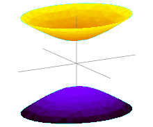
In simple terms, with two receivers at known locations, an emitter can be located onto a hyperboloid.^[1] Note that the receivers do not need to know the absolute time at which the pulse was transmitted – only the time difference is needed.

Consider now a third receiver at a third location. This would provide one extra independed TDOA measurement (there is a third TDOA, but this is dependend on the first two TDOA and does not provide extra information) and the emitter is located on the curve determined by the two intersecting hyperboloids. A fourth receiver is needed for another independed TDOA, this wil give an extra hyperboloid, the intersection of the curve with this hyperboloid gives one or two solutions, the emitter is then located at the one or at the one of the two solutions.

With four receivers there are 3 independend TDOA, three independend parameters are needed for a point in three dimensional space. (And for most constallations, three indendend TDOA will still give two points in 3D space). With additional receivers enhanced accuracy can be obtained. (Specifically for GPS the atmosphere does influence the traveling time of the signal and more satellites does give a more accurate location). For an overdetermined constallation (more than 4) a least squares can be used for 'reducing' the errors. extended Kalman filter are used for improving the individual signal timings. Averaging over longer times, can also improve accuracy.

The accuracy also improves if the receivers are placed in a configuration that minimizes the error of the estimate of the position.^[2]

The emitting platform may, or may not, cooperate in the multilateration surveillance processes.

Navigation application: locating a receiver from multiple transmitter sites

Multilateration can also be used by a single receiver to locate itself, by measuring signals emitted from three or more synchronized transmitters at known locations. At least three emitters are needed for two-dimensional navigation; at least four emitters are needed for three-dimensional navigation. For expository purposes, the emitters may be regarded as each broadcasting pulses at exactly the same time on a separate frequencies (to avoid interference). In this situation, the receiver measures the TDOAs of the pulses, which are converted to range differences.

However, operational systems are more complex. These methods have been implemented: (a) pulses are broadcast by different emitters on the same frequency, with known delays between transmission times; (b) continuous signals are broadcast on different frequencies, and their measured phase differences are converted to range differences; and (c) continuous signals are broadcast on the same carrier frequency, but each emitter modulates the carrier with a unique, known code. Correlation processing is used to obtain TDOAs.

The multilateration technique is used by several navigation systems. An historic example is the British DECCA system, developed during World War II. Decca used the phase-difference of three transmitters (method (b)). LORAN-C, introduced in the late 1950s, uses method (a). A current example is the Global Positioning System, or GPS. All GPS satellites broadcast on the same carrier frequency, which is modulated by pseudorandom codes (method (c)).

TDOA geometry

Rectangular/Cartesian coordinates

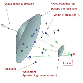
Geometry of spherical waves emanating from an emitter and passing through several receivers.

Fig 2. TDOA geometry.

Consider an emitter (E in Figure 2) at an unknown location vector

{\vec E}=(x,\,y,\,z)

which we wish to locate. The source is within range of N+1 receivers at known locations

{\vec P}_{0},\,{\vec P}_{1},\,\cdots ,\,{\vec P}_{m},\,\cdots ,\,{\vec P}_{N}.

The subscript m refers to any one of the receivers:

{\vec P}_{m}=(x_{m},\,y_{m},\,z_{m})

0 ≤ m ≤ N

The distance (R_m) from the emitter to one of the receivers in terms of the coordinates is

$R_{m}=\left|{\vec P}_{{m}}-{\vec E}\right|={\sqrt {(x_{m}-x)^{2}+(y_{m}-y)^{2}+(z_{m}-z)^{2}}}$

(1)

For some solution algorithms, the math is made easier by placing the origin at one of the receivers (P₀), which makes its distance to the emitter

$R_{0}={\sqrt {x^{2}+y^{2}+z^{2}}}$

(2)

Spherical coordinates

Low-frequency radio waves follow the curvature of the earth rather than a straight line. In this situation, equation 1 is not valid. LORAN-C and Omega are primary examples of systems that utilize spherical (vice slant) ranges. When a spherical model for the earth is satisfactory, the simplest expression for the central angle (sometimes termed the geocentric angle) between vehicle v and station m is

\cos \sigma _{{vm}}=\sin \phi _{v}\sin \phi _{m}+\cos \phi _{v}\cos \phi _{m}\cos \lambda _{{vm}}.

Here: latitudes are denoted by φ; longitudes are denoted by λ; and λ_vm = λ_v − λ_m. Alternative, better numerically behaved equivalent expressions, can be found in Great-circle navigation.

The distance R_m from the vehicle to station m is along a great circle will then be

R_{{m}}=R_{{E}}\sigma _{{vm}}

Here R_E is the assumed radius of the earth and σ_vm is expressed in radians.

Measuring the time difference in a TDOA system

Fig 3a. Pulse Signal

Fig 3b. Wide-band Signal

Fig 3c. Narrow-band Signal

Examples of measuring time difference with cross correlation.

The distance $R_{m}$ in equation 1 is the wave speed ( $v$ ) times transit time ( $T_{m}$ ). A TDOA multilateration system measures the time difference ( $\tau _{m}$ ) of a wavefront touching each receiver. The TDOA equation for receivers m and 0 is

${\begin{aligned}v\tau _{m}&=vT_{m}-vT_{0}\\v\tau _{m}&=R_{m}-R_{0}\end{aligned}}$

(3)

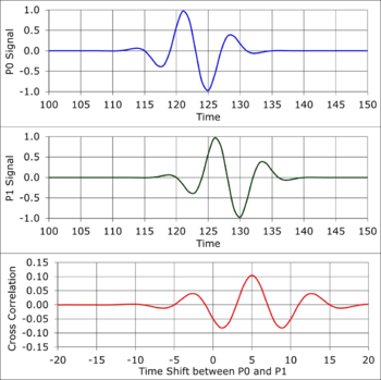
Figure 3a is a simulation of a pulse waveform recorded by receivers $P_{0}$ and $P_{1}$ . The spacing between $E$ , $P_{1}$ and $P_{0}$ is such that the pulse takes 5 time units longer to reach $P_{1}$ than $P_{0}$ . The units of time in Figure 3 are arbitrary. The following table gives approximate time scale units for recording different types of waves.

Type of wave	Material	Time Units
Acoustic	Air	1 millisecond
Acoustic	Water	1/2 millisecond
Acoustic	Rock	1/10 millisecond
Electromagnetic	Vacuum, air	1 nanosecond

The red curve in Figure 3a is the cross-correlation function $(P_{1}\star P_{0})$ . The cross correlation function slides one curve in time across the other and returns a peak value when the curve shapes match. The peak at time = 5 is a measure of the time shift between the recorded waveforms, which is also the $\tau$ value needed for Equation 3.

Figure 3b is the same type of simulation for a wide-band waveform from the emitter. The time shift is 5 time units because the geometry and wave speed is the same as the Figure 3a example. Again, the peak in the cross correlation occurs at $\tau _{1}=5$ .

Figure 3c is an example of a continuous, narrow-band waveform from the emitter. The cross correlation function shows an important factor when choosing the receiver geometry. There is a peak at Time = 5 plus every increment of the waveform period. To get one solution for the measured time difference, the largest space between any two receivers must be closer than one wavelength of the emitter signal. Some systems, such as the LORAN C and Decca mentioned at earlier (recall the same math works for moving receiver & multiple known transmitters), use spacing larger than 1 wavelength and include equipment, such as a Phase Detector, to count the number of cycles that pass by as the emitter moves. This only works for continuous, narrow-band waveforms because of the relation between phase ( $\theta$ ), frequency (f) and time (T)

\theta =2\pi f\cdot T

The phase detector will see variations in frequency as measured phase noise, which will be an uncertainty that propagates into the calculated location. If the phase noise is large enough, the phase detector can become unstable.

Solution algorithms

Overview

Equation 3 is the hyperboloid described in the previous section, where 4 receivers (0 ≤ m ≤ 3) lead to 3 non-linear equations in 3 unknown values (x,y,z). The system must then solve for the unknown emitter location in real time. Civilian air traffic control multilateration systems use the Mode C SSR transponder return to find the altitude. Three or more receivers at known locations are used to find the other two dimensions—either (x,y) for an airport application, or latitude and longitude for larger areas.

S. Bancroft first published the algebraic solution to the problem of locating a receiver using TDOA measurements involving 4 transmitters.^[3] Bancroft's algorithm reduces the problem to the solution of a quadratic equation, and yields the three Cartesian coordinates of the receiver as well as the common time of signal transmission. Other, comparable solutions and extensions were subsequently developed.^[4]^[5] The latter reference provides the solution for locating an aircraft with known altitude using TDOA measurements at 3 receivers.

When there are more measurements equations than unknown quantities (over-determined situation), the iterative Gauss-Newton algorithm for solving Non-linear least squares(NLLS) problems is generally preferred.^[6] An over-determined situation eliminates the possibility of ambiguous and/or extraneous solutions that can occur when only the minimum required number of measurements are available. The Gauss-Newton method may also be used with the minimum number of measurements — e.g., when an ellipsoidal model for earth must be employed. Since it is iterative, the Gauss-Newton method requires an initial solution estimate (which can be generated using a spherical earth model).

Multilateration systems employing spherical-range measurements utilize a combination of solution algorithms based on spherical trigonometry^[7] and the Gauss-Newton NLLS method.

Solution with limited computational resources

Improving accuracy with a large number of receivers can be a problem for devices with small embedded processors because of the time required to solve several simultaneous, non-linear equations (1, 2 & 3). The TDOA problem can be turned into a system of linear equations when there are 3 or more receivers, which can reduce the computation time. Starting with equation 3, solve for R_m, square both sides, collect terms and divide all terms by $v\tau _{m}$ :

${\begin{aligned}R_{{m}}^{2}&=(v\tau _{{m}}+R_{{0}})^{2}\\R_{{m}}^{2}&=(v\tau _{{m}})^{2}+2v\tau _{{m}}R_{{0}}+R_{{0}}^{2}\\0&=(v\tau _{{m}})^{2}+2v\tau _{{m}}R_{{0}}+R_{{0}}^{2}-R_{{m}}^{2}\\0&=(v\tau _{{m}})+2R_{{0}}+{\frac {(R_{{0}}^{2}-R_{{m}}^{2})}{v\tau _{{m}}}}.\\\end{aligned}}$

(4)

Removing the 2 R₀ term will eliminate all the square root terms. That is done by subtracting the TDOA equation of receiver m = 1 from each of the others (2 ≤ m ≤ N)

${\begin{aligned}&0=v\tau _{{m}}+2R_{{0}}+{\frac {(R_{{0}}^{2}-R_{{m}}^{2})}{v\tau _{{m}}}}\\&0=-v\tau _{{1}}-2R_{{0}}-{\frac {(R_{{0}}^{2}-R_{{1}}^{2})}{v\tau _{{1}}}}\\\hline \\&0=v\tau _{{m}}-v\tau _{{1}}+{\frac {(R_{{0}}^{2}-R_{{m}}^{2})}{v\tau _{{m}}}}-{\frac {(R_{{0}}^{2}-R_{{1}}^{2})}{v\tau _{{1}}}}.\end{aligned}}$

(5)

Focus for a moment on equation 1. Square R_m, group similar terms and use equation 2 to replace some of the terms with R₀.

${\begin{aligned}R_{m}^{2}&=x_{m}^{2}+y_{m}^{2}+z_{m}^{2}-x\ 2x_{m}-y\ 2y_{m}-z\ 2z_{m}+x^{2}+y^{2}+z^{2}\\&=x_{m}^{2}+y_{m}^{2}+z_{m}^{2}-x\ 2x_{m}-y\ 2y_{m}-z\ 2z_{m}+R_{0}^{2}\\R_{0}^{2}-R_{m}^{2}&=-x_{m}^{2}-y_{m}^{2}-z_{m}^{2}+x\ 2x_{m}+y\ 2y_{m}+z\ 2z_{m}.\end{aligned}}$

(6)

Combine equations 5 and 6, and write as a set of linear equations of the unknown emitter location x,y,z

${\begin{aligned}0&=xA_{m}+yB_{m}+zC_{m}+D_{m}\\&A_{m}={\frac {2x_{m}}{v\tau _{m}}}-{\frac {2x_{1}}{v\tau _{1}}}\\&B_{m}={\frac {2y_{m}}{v\tau _{m}}}-{\frac {2y_{1}}{v\tau _{1}}}\\&C_{m}={\frac {2z_{m}}{v\tau _{m}}}-{\frac {2z_{1}}{v\tau _{1}}}\\&D_{m}=v\tau _{m}-v\tau _{1}-{\frac {x_{m}^{2}+y_{m}^{2}+z_{m}^{2}}{v\tau _{m}}}+{\frac {x_{1}^{2}+y_{1}^{2}+z_{1}^{2}}{v\tau _{1}}}.\end{aligned}}$

(7)

Use equation 7 to generate the four constants $A_{m},B_{m},C_{m},D_{m}$ from measured distances and time for each receiver 2 ≤ m ≤ N. This will be a set of N-1 inhomogeneous linear equations.

There are many robust linear algebra methods that can solve for the values of (x,y,z), such as Gaussian Elimination. Chapter 15 in Numerical Recipes^[8] describes several methods to solve linear equations and estimate the uncertainty of the resulting values.

Two-dimensional solution

For finding the emitter location in a two dimensional geometry, one can generally adapt the methods used for the 3-D geometry. Additionally, there are specialized algorithms for two-dimensions—notable are the methods published by Fang^[9] (for a Cartesian plane) and Razin^[7] (for spherical earth).

When necessitated by the combination of vehicle-station distance (e.g., hundreds of miles or more) and required solution accuracy (e.g., less that 0.3% of the vehicle-stations distance), the ellipsoidal shape of the earth must be considered. This has been accomplished using the Gauss-Newton LLS method in conjunction with ellipsoid algorithms by Andoyer,^[10] Vincenty^[11] and Sodano.^[12]

Examples of 2-D multilateration are short wave radio long distance communications through the Earth's atmosphere, acoustic wave propagation in the sound fixing and ranging channel of the oceans and the LORAN navigation system.

Accuracy

For trilateration or multilateration, calculation is done based on distances, which requires the frequency and the wave count of a received transmission. For triangulation or multiangulation, calculation is done based on angles, which requires the phases of received transmission plus the wave count.

For lateration compared to angulation, the numerical problems compare, but the technical problem is more challenging with angular measurements, as angles require two measures per position when using optical or electronic means for measuring phase differences instead of counting wave cycles.

Trilateration in general is calculating with triangles of known distances/sizes, mathematically a very sound system. In a triangle, the angles can be derived if one knows the length of all sides, (see congruence), but the length of the sides cannot be derived based on all of the angles, not without knowing the length of at least one of the sides (a baseline) (see similarity).

In 3D, when four or more angles are in play, locations can be calculated from n + 1 = 4 measured angles plus one known baseline or from just n + 1 = 4 measured sides.

Multilateration is, in general, far more accurate for locating an object than sparse approaches such as trilateration, where with planar problems just three distances are known and computed. Multilateration serves for several aspects:

over-determination of an n-variable quadratic problem with (n + 1) + m quadratic equations
stochastic errors prohibiting a deterministic approach to solving the equations
clustering needs to segregate members of various clusters contributing to various models of solving, i.e. fixed locations, oscillating locations and moving locations

Accuracy of multilateration is a function of several variables, including:

The antenna or sensor geometry of the receiver(s) and transmitter(s) for electronic or optical transmission.
The timing accuracy of the receiver system, i.e. thermal stability of the clocking oscillators.
The accuracy of frequency synchronisation of the transmitter oscillators with the receiver oscillators.
Phase synchronisation of the transmitted signal with the received signal, as propagation effects as e.g. diffraction or reflection changes the phase of the signal thus indication deviation from line of sight, i.e. multipath reflections.
The bandwidth of the emitted pulse(s) and thus the rise-time of the pulses with pulse coded signals in transmission.
Inaccuracies in the locations of the transmitters or receivers when used as a known location

The accuracy can be calculated by using the Cramér–Rao bound and taking account of the above factors in its formulation. Additionally, a configuration of the sensors that minimizes a metric obtained from the Cramér–Rao bound can be chosen so as to optimize the actual position estimation of the target in a region of interest.^[2]

Example applications

Sound ranging – Using sound to locate artillery fire.
Electronic targets – Using the Mach wave of a bullet passing a sensor array to determine the point of arrival of the bullet on a firing range target.
Decca Navigator System – A system used from the end of World War II to the year 2000, employing the phase-difference of multiple transmitters to locate on the intersection of hyperboloids
OMEGA Navigation System – A worldwide system similar to Decca, shut down in 1997
GEE – British aircraft location technique from World War II, using accurate reference transmitters
LORAN-C – Navigation system using TDOA of signals from multiple synchronised transmitters
Passive ESM multilateration systems, including Kopáč, Ramona, Tamara, VERA and possibly Kolchuga – location of a transmitter using multiple receivers
Mobile phone tracking – using multiple base stations to estimate phone location (by either the phone itself, or the phone network)
Reduced Vertical Separation Minima (RVSM) monitoring using Secondary Surveillance Radar – Mode C/S transponder replies to calculate the position of an aircraft. Application to RVSM was first demonstrated by Roke Manor Research Limited in 1989.^[13]
Wide area multilateration (WAM) -- Surveillance system for airborne aircraft that measures the TDOA of emissions from the aircraft transponder (on 1090 MHz); in operational service in several countries
Airport Surface Detection Equipment, Model X (ASDE-X) -- Surveillance system for aircraft and other vehicles on the surface of an airport; includes a multilateration sub-system that measures the TDOA of emissions from the aircraft transponder (on 1090 MHz); ASDE-X is U.S. FAA terminology, equivalent systems are in operational service in several countries.

Simplification

For applications where no need for absolute coordinates determination is assessed, the implementing of a more simple solution is advantageous. Compared to multilateration as the concept of crisp locating, the other option is fuzzy locating, where just one distance delivers the relation between detector and detected object. This most simple approach is unilateration. However, such unilateration approach never delivers the angular position with reference to the detector. Many solutions are available today. Some of these vendors offer a position estimate based on combining several laterations. This approach is often not stable, when the wireless ambience is affected by metal or water masses. Other vendors offer room discrimination with a room-wise excitation, one vendor offers a position discrimination with a contiguity excitation.

Notes

↑ In other words, given two receivers at known locations, one can derive a three-dimensional surface (characterized as one half of a hyperboloid) for which any two points on said surface will have the same differential distance from said receivers, i.e., a signal transmitted from any point on the surface will have the same TDOA (measured by the receivers) as a signal transmitted from any other point on the surface.
Therefore, in practice, the TDOA corresponding to a (moving) transmitter is measured, a corresponding hyperbolic surface is derived, and the transmitter is said to be "located" somewhere on that surface.
1 2 Domingo-Perez, Francisco; Lazaro-Galilea, Jose Luis; Wieser, Andreas; Martin-Gorostiza, Ernesto; Salido-Monzu, David; Llana, Alvaro de la (April 2016). "Sensor placement determination for range-difference positioning using evolutionary multi-objective optimization". Expert Systems with Applications. 47: 95–105. doi:10.1016/j.eswa.2015.11.008.
↑ An Algebraic Solution of the GPS Equations, Stephen Bancroft, IEEE Transactions on Aerospace and Electronic Systems, Volume: AES-21, Issue: 1 (Jan. 1989), Pages 56-59.
↑ A Synthesizable VHDL Model of the Exact Solution for Three-dimensional Hyperbolic Positioning System, Ralph Bucher and D. Misra, VLSI Design, Volume 15 (2002), Issue 2, Pages 507-520.
↑ Aircraft Navigation and Surveillance Analysis for a Spherical Earth, Michael Geyer, John A. Volpe National Transportation Systems Center (U.S.), Oct. 2014, Section 7.4.
↑ Closed-form Algorithms in Mobile Positioning: Myths and Misconceptions, Niilo Sirola, Proceedings of the 7th Workshop on Positioning, Navigation and Communication 2010 (WPNC'10), March 11, 2010.
1 2 Explicit (Noniterative) Loran Solution, Sheldon Razin, Navigation: Journal of the Institute of Navigation, Vol. 14, No. 3, Fall 1967, pp. 265-269.
↑ Numerical Recipes official website
↑ Simple Solutions for Hyperbolic and Related Position Fixes, Bertrand T. Fang, IEEE Transactions on Aerospace and Electronic Systems, September 1990, pp 748-753
↑ Formule donnant la longueur de la géodésique, joignant 2 points de l'ellipsoide donnes par leurs coordonnées geographiques, Marie Henri Andoyer, Bulletin Geodsique, No. 34 (1932), pages 77-81
↑ Direct and Inverse Solutions of Geodesics on the Ellipsoids with Applications of Nested Equations, Thaddeus Vincenty, Survey Review, XXIII, Number 176 (April 1975)
↑ General non-iterative solution of the inverse and direct geodetic problems, Emanuel M. Sodano, Bulletin Géodésique, vol 75 (1965), pp 69-89
↑ Air Traffic Technology International (2002). "Perfect Timing" (PDF). Retrieved 31 August 2012.

References

The Multilateration Executive Reference Guide is an easy-to-read reference for air traffic management, airport and airline professionals to learn more about this next-generation surveillance technology

This article is issued from Wikipedia - version of the 11/7/2016. The text is available under the Creative Commons Attribution/Share Alike but additional terms may apply for the media files.