Maxwell–Boltzmann distribution

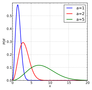
Not to be confused with Maxwell–Boltzmann statistics.

Maxwell–Boltzmann
Probability density function
Cumulative distribution function
Parameters	$a>0$
Support	$x\in (0;\infty)$
PDF	$\sqrt{\frac{2}{\pi}} \frac{x^2 e^{-x^2/\left(2a^2\right)}}{a^3}$
CDF	$\operatorname{erf}\left(\frac{x}{\sqrt{2} a}\right) -\sqrt{\frac{2}{\pi}} \frac{x e^{-x^2/\left(2a^2\right)}}{a}$ where erf is the error function
Mean	$\mu=2a \sqrt{\frac{2}{\pi}}$
Mode	$\sqrt{2} a$
Variance	$\sigma^2=\frac{a^2(3 \pi - 8)}{\pi}$
Skewness	$\gamma_1=\frac{2 \sqrt{2} (16 -5 \pi)}{(3 \pi - 8)^{3/2}}$
Ex. kurtosis	$\gamma_2=4\frac{\left(-96+40\pi-3\pi^2\right)}{(3 \pi - 8)^2}$
Entropy	$\ln\left(a\sqrt{2\pi}\right)+\gamma-\frac{1}{2}$

In statistics the Maxwell–Boltzmann distribution is a particular probability distribution named after James Clerk Maxwell and Ludwig Boltzmann. It was first defined and used in physics (in particular in statistical mechanics) for describing particle speeds in idealized gases where the particles move freely inside a stationary container without interacting with one another, except for very brief collisions in which they exchange energy and momentum with each other or with their thermal environment. Particle in this context refers to gaseous particles (atoms or molecules), and the system of particles is assumed to have reached thermodynamic equilibrium.^[1] While the distribution was first derived by Maxwell in 1860 on heuristic grounds,^[2] Boltzmann later carried out significant investigations into the physical origins of this distribution.

A particle speed probability distribution indicates which speeds are more likely: a particle will have a speed selected randomly from the distribution, and is more likely to be within one range of speeds than another. The distribution depends on the temperature of the system and the mass of the particle.^[3] The Maxwell–Boltzmann distribution applies to the classical ideal gas, which is an idealization of real gases. In real gases, there are various effects (e.g., van der Waals interactions, vortical flow, relativistic speed limits, and quantum exchange interactions) that can make their speed distribution different from the Maxwell–Boltzmann form. However, rarefied gases at ordinary temperatures behave very nearly like an ideal gas and the Maxwell speed distribution is an excellent approximation for such gases. Thus, it forms the basis of the Kinetic theory of gases, which provides a simplified explanation of many fundamental gaseous properties, including pressure and diffusion.^[4]

Distribution function

The speed probability density functions of the speeds of a few noble gases at a temperature of 298.15 K (25 °C). The y-axis is in s/m so that the area under any section of the curve (which represents the probability of the speed being in that range) is dimensionless.

The Maxwell–Boltzmann distribution is the function^[5]

f(v) = \sqrt{\left(\frac{m}{2 \pi kT}\right)^3}\, 4\pi v^2 e^{- \frac{mv^2}{2kT}},

where $m$ is the particle mass and $kT$ is the product of Boltzmann's constant and thermodynamic temperature.

This probability density function gives the probability, per unit speed, of finding the particle with a speed near $v$ . This equation is simply the Maxwell distribution (given in the infobox) with distribution parameter $a=\sqrt{kT/m}$ . In probability theory the Maxwell–Boltzmann distribution is a chi distribution with three degrees of freedom and scale parameter $a=\sqrt{kT/m}$ .

The simplest ordinary differential equation satisfied by the distribution is:

kTvf'(v)+f(v)(mv^{2}-2kT)=0,

f(1)={\sqrt {{\frac {2}{\pi }}}}e^{{-{\frac {m}{2kT}}}}\left({\frac {m}{kT}}\right)^{{3/2}}

or in unitless presentation:

a^{2}xf'(x)+\left(x^{2}-2a^{2}\right)f(x)=0,

f(1)={\frac {{\sqrt {{\frac {2}{\pi }}}}e^{{-{\frac {1}{2a^{2}}}}}}{a^{3}}}.

Note that a distribution (function) is not the same as the probability. The distribution (function) stands for an average number, as in all three kinds of statistics (Maxwell–Boltzmann, Bose–Einstein, Fermi–Dirac). With the Darwin–Fowler method of mean values the Maxwell–Boltzmann distribution is obtained as an exact result.

Typical speeds

The mean speed, most probable speed (mode), and root-mean-square can be obtained from properties of the Maxwell distribution.

The most probable speed, v_p, is the speed most likely to be possessed by any molecule (of the same mass m) in the system and corresponds to the maximum value or mode of f(v). To find it, we calculate the derivative df/dv, set it to zero and solve for v:
$\frac{df(v)}{dv} = 0$

which yields:

$v_p = \sqrt { \frac{2kT}{m} } = \sqrt { \frac{2RT}{M} }$

where R is the gas constant and M = N_A m is the molar mass of the substance.
For diatomic nitrogen (N₂, the primary component of air) at room temperature (300 K), this gives $v_p = 422$ m/s
The mean speed is the expected value of the speed distribution
$\langle v \rangle = \int_0^{\infty} v \, f(v) \, dv= \sqrt { \frac{8kT}{\pi m}}= \sqrt { \frac{8RT}{\pi M}} = \frac{2}{\sqrt{\pi}} v_p$
The root mean square speed is the second-order moment of speed:
$\sqrt{\langle v^2 \rangle} = \left(\int_0^{\infty} v^2 \, f(v) \, dv \right)^{1/2}= \sqrt { \frac{3kT}{m}}= \sqrt { \frac{3RT}{M} } = \sqrt{ \frac{3}{2} } v_p$

The typical speeds are related as follows:

0.886 \langle v \rangle = v_p < \langle v \rangle < \sqrt{\langle v^2 \rangle} = 1.085 \langle v \rangle.

Derivation and related distributions

The original derivation in 1860 by James Clerk Maxwell was an argument based on demanding certain symmetries in the speed distribution function.^[2] After Maxwell, Ludwig Boltzmann in 1872 derived the distribution on more mechanical grounds by using the assumptions of his Kinetic theory of gases, and showed that gases should over time tend toward this distribution, due to collisions (see H-theorem). He later (1877) derived the distribution again under the framework of statistical thermodynamics. The derivations in this section are along the lines of Boltzmann's 1877 derivation, starting with result known as Maxwell–Boltzmann statistics (from statistical thermodynamics). Maxwell–Boltzmann statistics gives the average number of particles found in a given single-particle microstate, under certain assumptions:^[1]^[6]

${\frac {N_{i}}{N}}={\frac {\exp(-E_{i}/kT)}{\sum _{j}\exp(-E_{j}/kT)}}$

(1)

where:

i and j are indices (or labels) of the single-particle micro states,
N_i is the average number of particles in the single-particle microstate i,
N is the total number of particles in the system,
E_i is the energy of microstate i,
T is the equilibrium temperature of the system,
k is the Boltzmann constant.

The assumptions of this equation are that the particles do not interact, and that they are classical; this means that each particle's state can be considered independently from the other particles' states. Additionally, the particles are assumed to be in thermal equilibrium. The denominator in Equation (1) is simply a normalizing factor so that the N_i/N add up to 1 — in other words it is a kind of partition function (for the single-particle system, not the usual partition function of the entire system).

Because velocity and speed are related to energy, Equation (1) can be used to derive relationships between temperature and the speeds of gas particles. All that is needed is to discover the density of microstates in energy, which is determined by dividing up momentum space into equal sized regions.

Distribution for the momentum vector

The potential energy is taken to be zero, so that all energy is in the form of kinetic energy. The relationship between kinetic energy and momentum for massive non-relativistic particles is

$E=\frac{p^2}{2m}$

(2)

where p² is the square of the momentum vector p = [p_x, p_y, p_z]. We may therefore rewrite Equation (1) as:

$\frac{N_i}{N} = \frac{1}{Z} \exp \left[ -\frac{p_{i, x}^2 + p_{i, y}^2 + p_{i, z}^2}{2mkT} \right]$

(3)

where Z is the partition function, corresponding to the denominator in Equation (1). Here m is the molecular mass of the gas, T is the thermodynamic temperature and k is the Boltzmann constant. This distribution of N_i/N is proportional to the probability density function f_p for finding a molecule with these values of momentum components, so:

$f_\mathbf{p} (p_x, p_y, p_z) = \frac{c}{Z} \exp \left[ -\frac{p_x^2 + p_y^2 + p_z^2}{2mkT} \right]$

(4)

The normalizing constant c, can be determined by recognizing that the probability of a molecule having some momentum must be 1. Therefore the integral of equation (4) over all p_x, p_y, and p_z must be 1.

It can be shown that:

$c = \frac{Z}{(2 \pi mkT)^{3/2}}$

(5)

Substituting Equation (5) into Equation (4) gives:

$f_\mathbf{p} (p_x, p_y, p_z) = \left( 2 \pi mkT \right)^{-3/2} \exp \left[ -\frac{p_x^2 + p_y^2 + p_z^2}{2mkT} \right]$ (6)

The distribution is seen to be the product of three independent normally distributed variables $p_{x}$ , $p_{y}$ , and $p_{z}$ , with variance $mkT$ . Additionally, it can be seen that the magnitude of momentum will be distributed as a Maxwell–Boltzmann distribution, with $a=\sqrt{mkT}$ . The Maxwell–Boltzmann distribution for the momentum (or equally for the velocities) can be obtained more fundamentally using the H-theorem at equilibrium within the Kinetic theory of gases framework.

Distribution for the energy

The energy distribution is found imposing

$f_{E}(E)dE=f_{p}({\textbf p})d^{3}{\textbf p},$

(7)

where $d^{3}{\textbf p}$ is the infinitesimal phase-space volume of momenta corresponding to the energy interval $dE$ . Making use of the spherical symmetry of the energy-momentum dispersion relation $E=|{\textbf p}|^{2}/2m$ , this can be expressed in terms of $dE$ as

$d^{3}{\textbf p}=4\pi |{\textbf p}|^{2}d|{\textbf p}|=4\pi m{\sqrt {2mE}}dE.$

(8)

Using then (8) in (7), and expressing everything in terms of the energy $E$ , we get

f_{E}(E)dE={\frac {1}{(2\pi mkT)^{{3/2}}}}e^{{-E/kT}}4\pi m{\sqrt {2mE}}dE=2{\sqrt {{\frac {E}{\pi }}}}\left({\frac {1}{kT}}\right)^{{3/2}}\exp \left({\frac {-E}{kT}}\right)dE

and finally

$f_{E}(E)=2{\sqrt {{\frac {E}{\pi }}}}\left({\frac {1}{kT}}\right)^{{3/2}}\exp \left({\frac {-E}{kT}}\right)$ (9)

Since the energy is proportional to the sum of the squares of the three normally distributed momentum components, this distribution is a gamma distribution; in particular, it is a chi-squared distribution with three degrees of freedom.

By the equipartition theorem, this energy is evenly distributed among all three degrees of freedom, so that the energy per degree of freedom is distributed as a chi-squared distribution with one degree of freedom:^[7]

f_{\epsilon }(\epsilon )\,d\epsilon ={\sqrt {\frac {1}{\pi \epsilon kT}}}~\exp \left[{\frac {-\epsilon }{kT}}\right]\,d\epsilon

where $\epsilon$ is the energy per degree of freedom. At equilibrium, this distribution will hold true for any number of degrees of freedom. For example, if the particles are rigid mass dipoles of fixed dipole moment, they will have three translational degrees of freedom and two additional rotational degrees of freedom. The energy in each degree of freedom will be described according to the above chi-squared distribution with one degree of freedom, and the total energy will be distributed according to a chi-squared distribution with five degrees of freedom. This has implications in the theory of the specific heat of a gas.

The Maxwell–Boltzmann distribution can also be obtained by considering the gas to be a type of quantum gas for which the approximation ε >> k T may be made.

Distribution for the velocity vector

Recognizing that the velocity probability density f_v is proportional to the momentum probability density function by

f_\mathbf{v} d^3v = f_\mathbf{p} \left(\frac{dp}{dv}\right)^3 d^3v

and using p = mv we get

$f_{{\mathbf {v}}}(v_{x},v_{y},v_{z})=\left({\frac {m}{2\pi kT}}\right)^{{3/2}}\exp \left[-{\frac {m(v_{x}^{2}+v_{y}^{2}+v_{z}^{2})}{2kT}}\right]$

which is the Maxwell–Boltzmann velocity distribution. The probability of finding a particle with velocity in the infinitesimal element [dv_x, dv_y, dv_z] about velocity v = [v_x, v_y, v_z] is

f_\mathbf{v} \left(v_x, v_y, v_z\right)\, dv_x\, dv_y\, dv_z.

Like the momentum, this distribution is seen to be the product of three independent normally distributed variables $v_x$ , $v_y$ , and $v_z$ , but with variance $\frac{kT}{m}$ . It can also be seen that the Maxwell–Boltzmann velocity distribution for the vector velocity [v_x, v_y, v_z] is the product of the distributions for each of the three directions:

f_v \left(v_x, v_y, v_z\right) = f_v (v_x)f_v (v_y)f_v (v_z)

where the distribution for a single direction is

f_v (v_i) = \sqrt{\frac{m}{2 \pi kT}} \exp \left[ \frac{-mv_i^2}{2kT} \right].

Each component of the velocity vector has a normal distribution with mean $\mu_{v_x} = \mu_{v_y} = \mu_{v_z} = 0$ and standard deviation $\sigma_{v_x} = \sigma_{v_y} = \sigma_{v_z} = \sqrt{\frac{kT}{m}}$ , so the vector has a 3-dimensional normal distribution, a particular kind of multivariate normal distribution, with mean $\mu_{\mathbf{v}} = {\mathbf{0}}$ and standard deviation $\sigma_{\mathbf{v}} = \sqrt{\frac{3kT}{m}}$ .

The Maxwell–Boltzmann distribution for the speed follows immediately from the distribution of the velocity vector, above. Note that the speed is

v = \sqrt{v_x^2 + v_y^2 + v_z^2}

and the volume element in spherical coordinates

dv_x\, dv_y\, dv_z = v^2 \sin \theta\, dv\, d\theta\, d\phi

where $\phi$ and $\theta$ are the "course" (azimuth of the velocity vector) and "path angle" (elevation angle of the velocity vector). Integration of the normal probability density function of the velocity, above, over the course (from 0 to $2\pi$ ) and path angle (from 0 to $\pi$ ), with substitution of the speed for the sum of the squares of the vector components, yields the speed distribution.

References

1 2 Statistical Physics (2nd Edition), F. Mandl, Manchester Physics, John Wiley & Sons, 2008, ISBN 9780471915331
1 2
See:
- Maxwell, J.C. (1860) "Illustrations of the dynamical theory of gases. Part I. On the motions and collisions of perfectly elastic spheres," Philosophical Magazine, 4th series, 19 : 19–32.
- Maxwell, J.C. (1860) "Illustrations of the dynamical theory of gases. Part II. On the process of diffusion of two or more kinds of moving particles among one another," Philosophical Magazine, 4th series, 20 : 21–37.
↑ University Physics – With Modern Physics (12th Edition), H.D. Young, R.A. Freedman (Original edition), Addison-Wesley (Pearson International), 1st Edition: 1949, 12th Edition: 2008, ISBN 978-0-321-50130-1
↑ Encyclopaedia of Physics (2nd Edition), R.G. Lerner, G.L. Trigg, VHC publishers, 1991, ISBN 3-527-26954-1 (Verlagsgesellschaft), ISBN 0-89573-752-3 (VHC Inc.)
↑ H.J.W. Müller-Kirsten, Basics of Statistical Physics, 2nd ed., World Scientific (2013),ISBN 978-981-4449-53-3, Chapter 2.
↑ McGraw Hill Encyclopaedia of Physics (2nd Edition), C.B. Parker, 1994, ISBN 0-07-051400-3
↑ Laurendeau, Normand M. (2005). Statistical thermodynamics: fundamentals and applications. Cambridge University Press. p. 434. ISBN 0-521-84635-8. , Appendix N, page 434

External links

"The Maxwell Speed Distribution" from The Wolfram Demonstrations Project at Mathworld

Probability distributions

List

Discrete univariate with finite support	Benford Bernoulli beta-binomial binomial categorical hypergeometric Poisson binomial Rademacher discrete uniform Zipf Zipf–Mandelbrot

Discrete univariate with infinite support	beta negative binomial Borel Conway–Maxwell–Poisson discrete phase-type Delaporte extended negative binomial Gauss–Kuzmin geometric logarithmic negative binomial parabolic fractal Poisson Skellam Yule–Simon zeta

Continuous univariate supported on a bounded interval	arcsine ARGUS Balding–Nichols Bates beta beta rectangular Irwin–Hall Kumaraswamy logit-normal noncentral beta raised cosine reciprocal triangular U-quadratic uniform Wigner semicircle

Continuous univariate supported on a semi-infinite interval	Benini Benktander 1st kind Benktander 2nd kind beta prime Burr chi-squared chi Dagum Davis exponential-logarithmic Erlang exponential F folded normal Flory–Schulz Fréchet gamma gamma/Gompertz generalized inverse Gaussian Gompertz half-logistic half-normal Hotelling's T-squared hyper-Erlang hyperexponential hypoexponential inverse chi-squared scaled inverse chi-squared inverse Gaussian inverse gamma Kolmogorov Lévy log-Cauchy log-Laplace log-logistic log-normal Lomax matrix-exponential Maxwell–Boltzmann Maxwell–Jüttner Mittag-Leffler Nakagami noncentral chi-squared Pareto phase-type poly-Weibull Rayleigh relativistic Breit–Wigner Rice shifted Gompertz truncated normal type-2 Gumbel Weibull Discrete Weibull Wilks's lambda

Continuous univariate supported on the whole real line	Cauchy exponential power Fisher's z Gaussian q generalized normal generalized hyperbolic geometric stable Gumbel Holtsmark hyperbolic secant Johnson's S_U Landau Laplace asymmetric Laplace logistic noncentral t normal (Gaussian) normal-inverse Gaussian skew normal slash stable Student's t type-1 Gumbel Tracy–Widom variance-gamma Voigt

Continuous univariate with support whose type varies	generalized extreme value generalized Pareto Tukey lambda q-Gaussian q-exponential q-Weibull shifted log-logistic

Mixed continuous-discrete univariate	rectified Gaussian

Multivariate (joint)	Discrete Ewens multinomial Dirichlet-multinomial negative multinomial Continuous Dirichlet generalized Dirichlet multivariate normal multivariate stable multivariate t normal-inverse-gamma normal-gamma Matrix-valued inverse matrix gamma inverse-Wishart matrix normal matrix t matrix gamma normal-inverse-Wishart normal-Wishart Wishart

Directional	Univariate (circular) directional Circular uniform univariate von Mises wrapped normal wrapped Cauchy wrapped exponential wrapped asymmetric Laplace wrapped Lévy Bivariate (spherical) Kent Bivariate (toroidal) bivariate von Mises Multivariate von Mises–Fisher Bingham

Degenerate and singular	Degenerate Dirac delta function Singular Cantor

Families	Circular compound Poisson elliptical exponential natural exponential location-scale maximum entropy mixture Pearson Tweedie wrapped

This article is issued from Wikipedia - version of the 10/4/2016. The text is available under the Creative Commons Attribution/Share Alike but additional terms may apply for the media files.