Matrix chain multiplication
Matrix chain multiplication (or Matrix Chain Ordering Problem, MCOP) is an optimization problem that can be solved using dynamic programming. Given a sequence of matrices, the goal is to find the most efficient way to multiply these matrices. The problem is not actually to perform the multiplications, but merely to decide the sequence of the matrix multiplications involved.
Here are many options because matrix multiplication is associative. In other words, no matter how the product is parenthesized, the result obtained will remain the same. For example, for four matrices A, B, C, and D, we would have:
- ((AB)C)D = ((A(BC))D) = (AB)(CD) = A((BC)D) = A(B(CD)).
However, the order in which the product is parenthesized affects the number of simple arithmetic operations needed to compute the product, or the efficiency. For example, if A is a 10 × 30 matrix, B is a 30 × 5 matrix, and C is a 5 × 60 matrix, then
- computing (AB)C needs (10×30×5) + (10×5×60) = 1500 + 3000 = 4500 operations, while
- computing A(BC) needs (30×5×60) + (10×30×60) = 9000 + 18000 = 27000 operations.
Clearly the first method is more efficient. With this information, the problem statement can be refined as "how to determine the optimal parenthesization of a product of n matrices?" Checking each possible parenthesization (brute force) would require a run-time that is exponential in the number of matrices, which is very slow and impractical for large n. A quicker solution to this problem can be achieved by breaking up the problem into a set of related subproblems. By solving subproblems once and reusing the solutions, the required run-time can drastically reduced. This concept is known as dynamic programming.
A dynamic programming algorithm
To begin, let us assume that all we really want to know is the minimum cost, or minimum number of arithmetic operations, needed to multiply out the matrices. If we are only multiplying two matrices, there is only one way to multiply them, so the minimum cost is the cost of doing this. In general, we can find the minimum cost using the following recursive algorithm:
- Take the sequence of matrices and separate it into two subsequences.
- Find the minimum cost of multiplying out each subsequence.
- Add these costs together, and add in the cost of multiplying the two result matrices.
- Do this for each possible position at which the sequence of matrices can be split, and take the minimum over all of them.
For example, if we have four matrices ABCD, we compute the cost required to find each of (A)(BCD), (AB)(CD), and (ABC)(D), making recursive calls to find the minimum cost to compute ABC, AB, CD, and BCD. We then choose the best one. Better still, this yields not only the minimum cost, but also demonstrates the best way of doing the multiplication: group it the way that yields the lowest total cost, and do the same for each factor.
However, if we implement this algorithm we discover that it is just as slow as the naive way of trying all permutations! What went wrong? The answer is that we're doing a lot of redundant work. For example, above we made a recursive call to find the best cost for computing both ABC and AB. But finding the best cost for computing ABC also requires finding the best cost for AB. As the recursion grows deeper, more and more of this type of unnecessary repetition occurs.
One simple solution is called memoization: each time we compute the minimum cost needed to multiply out a specific subsequence, we save it. If we are ever asked to compute it again, we simply give the saved answer, and do not recompute it. Since there are about n2/2 different subsequences, where n is the number of matrices, the space required to do this is reasonable. It can be shown that this simple trick brings the runtime down to O(n3) from O(2n), which is more than efficient enough for real applications. This is top-down dynamic programming.
The following bottom-up approach [1] computes, for each 2 ≤ k ≤ n, the minimum costs of all subsequences of length k, using the costs of smaller subsequences already computed. It has the same asymptotic runtime and requires no recursion.
Pseudocode:
// Matrix A[i] has dimension dims[i-1] x dims[i] for i = 1..n
MatrixChainOrder(int dims[])
{
    // length[dims] = n + 1
    n = dims.length - 1;
    // m[i,j] = Minimum number of scalar multiplications (i.e., cost)
    // needed to compute the matrix A[i]A[i+1]...A[j] = A[i..j]
    // The cost is zero when multiplying one matrix
    for (i = 1; i <= n; i++)
        m[i, i] = 0;

    for (len = 2; len <= n; len++) { // Subsequence lengths
        for (i = 1; i <= n - len + 1; i++) {
            j = i + len - 1;
            m[i, j] = MAXINT;
            for (k = i; k <= j - 1; k++) {
                cost = m[i, k] + m[k+1, j] + dims[i-1]*dims[k]*dims[j];
                if (cost < m[i, j]) {
                    m[i, j] = cost;
                    s[i, j] = k; // Index of the subsequence split that achieved minimal cost
                }
            }
        }
    }
}
- Note : The first index for dims is 0 and the first index for m and s is 1
A java implementation using zero based array indexes along with a convenience method for printing the solved order of operations:
public class MatrixOrderOptimization {
    protected int[][]m;
    protected int[][]s;
    public void matrixChainOrder(int[] dims) {
        int n = dims.length - 1;
        m = new int[n][n];
        s = new int[n][n];

        for (int lenMinusOne = 1; lenMinusOne < n; lenMinusOne++) {
            for (int i = 0; i < n - lenMinusOne; i++) {
                int j = i + lenMinusOne;
                m[i][j] = Integer.MAX_VALUE;
                for (int k = i; k < j; k++) {
                    int cost = m[i][k] + m[k+1][j] + dims[i]*dims[k+1]*dims[j+1];
                    if (cost < m[i][j]) {
                        m[i][j] = cost;
                        s[i][j] = k;
                    }
                }
            }
        }
    }

    public void printOptimalParenthesizations() {
        boolean[] inAResult = new boolean[s.length];
        printOptimalParenthesizations(s, 0, s.length - 1, inAResult);
    }

    void printOptimalParenthesizations(int[][]s, int i, int j,  /* for pretty printing: */ boolean[] inAResult) {
        if (i != j) {
            printOptimalParenthesizations(s, i, s[i][j], inAResult);
            printOptimalParenthesizations(s, s[i][j] + 1, j, inAResult);
            String istr = inAResult[i] ? "_result " : " ";
            String jstr = inAResult[j] ? "_result " : " ";
            System.out.println(" A_" + i + istr + "* A_" + j + jstr);
            inAResult[i] = true;
            inAResult[j] = true;
        }
    }
}
At the end of this program, we have the minimum cost for the full sequence.
More efficient algorithms
There are algorithms that are more efficient than the O(n3) dynamic programming algorithm, though they are more complex.
Hu & Shing (1981)
An algorithm published in 1981 by Hu and Shing achieves O(n log n) complexity.[2][3][4] They showed how the matrix chain multiplication problem can be transformed (or reduced) into the problem of triangulation of a regular polygon. The polygon is oriented such that there is a horizontal bottom side, called the base, which represents the final result. The other n sides of the polygon, in the clockwise direction, represent the matrices. The vertices on each end of a side are the dimensions of the matrix represented by that side. With n matrices in the multiplication chain there are n−1 binary operations and Cn−1 ways of placing parenthesizes, where Cn−1 is the (n−1)-th Catalan number. The algorithm exploits that there are also Cn−1 possible triangulations of a polygon with n+1 sides.
This image illustrates possible triangulations of a regular hexagon. These correspond to the different ways that parentheses can be placed to order the multiplications for a product of 5 matrices.

For the example below, there are four sides: A, B, C and the final result ABC. A is a 10×30 matrix, B is a 30×5 matrix, C is a 5×60 matrix, and the final result is a 10×60 matrix. The regular polygon for this example is a 4-gon, i.e. a square:

The matrix product AB is a 10x5 matrix and BC is a 30x60 matrix. The two possible triangulations in this example are:
-

Polygon representation of (AB)C
-
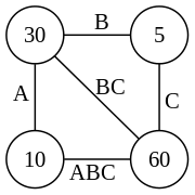
Polygon representation of A(BC)
The cost of a single triangle in terms of the number of multiplications needed is the product of its vertices. The total cost of a particular triangulation of the polygon is the sum of the costs of all its triangles:
- (AB)C: (10×30×5) + (10×5×60) = 1500 + 3000 = 4500 multiplications
- A(BC): (30×5×60) + (10×30×60) = 9000 + 18000 = 27000 multiplications
Hu & Shing developed an algorithm that finds an optimum solution for the minimum cost partition problem in O(n log n) time.
Generalizations
The matrix chain multiplication problem generalizes to solving a more abstract problem: given a linear sequence of objects, an associative binary operation on those objects, and a way to compute the cost of performing that operation on any two given objects (as well as all partial results), compute the minimum cost way to group the objects to apply the operation over the sequence.[5] One somewhat contrived special case of this is string concatenation of a list of strings. In C, for example, the cost of concatenating two strings of length m and n using strcat is O(m + n), since we need O(m) time to find the end of the first string and O(n) time to copy the second string onto the end of it. Using this cost function, we can write a dynamic programming algorithm to find the fastest way to concatenate a sequence of strings. However, this optimization is rather useless because we can straightforwardly concatenate the strings in time proportional to the sum of their lengths. A similar problem exists for singly linked lists.
Another generalization is to solve the problem when parallel processors are available. In this case, instead of adding the costs of computing each factor of a matrix product, we take the maximum because we can do them simultaneously. This can drastically affect both the minimum cost and the final optimal grouping; more "balanced" groupings that keep all the processors busy are favored. There are even more sophisticated approaches.[6]
References
- ↑ Cormen, Thomas H; Leiserson, Charles E; Rivest, Ronald L; Stein, Clifford (2001). "15.2: Matrix-chain multiplication". Introduction to Algorithms. Second Edition. MIT Press and McGraw-Hill. pp. 331–338. ISBN 0-262-03293-7.
- ↑ Hu, TC; Shing, MT (1981). Computation of Matrix Chain Products, Part I, Part II (PDF) (Technical report). Stanford University, Department of Computer Science. STAN-CS-TR-81-875.
- ↑ Hu, TC; Shing, MT (1982). "Computation of Matrix Chain Products, Part I" (PDF). SIAM Journal on Computing. Society for Industrial and Applied Mathematics. 11 (2): 362–373. doi:10.1137/0211028. ISSN 0097-5397.
- ↑ Hu, TC; Shing, MT (1984). "Computation of Matrix Chain Products, Part II" (PDF). SIAM Journal on Computing. Society for Industrial and Applied Mathematics. 13 (2): 228–251. doi:10.1137/0213017. ISSN 0097-5397.
- ↑ G. Baumgartner, D. Bernholdt, D. Cociorva, R. Harrison, M. Nooijen, J. Ramanujam and P. Sadayappan. A Performance Optimization Framework for Compilation of Tensor Contraction Expressions into Parallel Programs. 7th International Workshop on High-Level Parallel Programming Models and Supportive Environments (HIPS '02). Fort Lauderdale, Florida. 2002 available at http://citeseer.ist.psu.edu/610463.html and at http://www.csc.lsu.edu/~gb/TCE/Publications/OptFramework-HIPS02.pdf
- ↑ Heejo Lee, Jong Kim, Sungje Hong, and Sunggu Lee. Processor Allocation and Task Scheduling of Matrix Chain Products on Parallel Systems. IEEE Trans. on Parallel and Distributed Systems, Vol. 14, No. 4, pp. 394–407, Apr. 2003