Mathematical model
A mathematical model is a description of a system using mathematical concepts and language. The process of developing a mathematical model is termed mathematical modeling. Mathematical models are used in the natural sciences (such as physics, biology, earth science, meteorology) and engineering disciplines (such as computer science, artificial intelligence), as well as in the social sciences (such as economics, psychology, sociology, political science). Physicists, engineers, statisticians, operations research analysts, and economists use mathematical models most extensively. A model may help to explain a system and to study the effects of different components, and to make predictions about behaviour.
Elements of a mathematical model
Mathematical models can take many forms, including dynamical systems, statistical models, differential equations, or game theoretic models. These and other types of models can overlap, with a given model involving a variety of abstract structures. In general, mathematical models may include logical models. In many cases, the quality of a scientific field depends on how well the mathematical models developed on the theoretical side agree with results of repeatable experiments. Lack of agreement between theoretical mathematical models and experimental measurements often leads to important advances as better theories are developed.
The traditional mathematical model contains four major elements. These are
Classifications
Mathematical models are usually composed of relationships and variables. Relationships can be described by operators, such as algebraic operators, functions, differential operators, etc. Variables are abstractions of system parameters of interest, that can be quantified. Several classification criteria can be used for mathematical models according to their structure:
- Linear vs. nonlinear: If all the operators in a mathematical model exhibit linearity, the resulting mathematical model is defined as linear. A model is considered to be nonlinear otherwise. The definition of linearity and nonlinearity is dependent on context, and linear models may have nonlinear expressions in them. For example, in a statistical linear model, it is assumed that a relationship is linear in the parameters, but it may be nonlinear in the predictor variables. Similarly, a differential equation is said to be linear if it can be written with linear differential operators, but it can still have nonlinear expressions in it. In a mathematical programming model, if the objective functions and constraints are represented entirely by linear equations, then the model is regarded as a linear model. If one or more of the objective functions or constraints are represented with a nonlinear equation, then the model is known as a nonlinear model.
Nonlinearity, even in fairly simple systems, is often associated with phenomena such as chaos and irreversibility. Although there are exceptions, nonlinear systems and models tend to be more difficult to study than linear ones. A common approach to nonlinear problems is linearization, but this can be problematic if one is trying to study aspects such as irreversibility, which are strongly tied to nonlinearity. - Static vs. dynamic: A dynamic model accounts for time-dependent changes in the state of the system, while a static (or steady-state) model calculates the system in equilibrium, and thus is time-invariant. Dynamic models typically are represented by differential equations.
- Explicit vs. implicit: If all of the input parameters of the overall model are known, and the output parameters can be calculated by a finite series of computations (known as linear programming, not to be confused with linearity as described above), the model is said to be explicit. But sometimes it is the output parameters which are known, and the corresponding inputs must be solved for by an iterative procedure, such as Newton's method (if the model is linear) or Broyden's method (if non-linear). For example, a jet engine's physical properties such as turbine and nozzle throat areas can be explicitly calculated given a design thermodynamic cycle (air and fuel flow rates, pressures, and temperatures) at a specific flight condition and power setting, but the engine's operating cycles at other flight conditions and power settings cannot be explicitly calculated from the constant physical properties.
- Discrete vs. continuous: A discrete model treats objects as discrete, such as the particles in a molecular model or the states in a statistical model; while a continuous model represents the objects in a continuous manner, such as the velocity field of fluid in pipe flows, temperatures and stresses in a solid, and electric field that applies continuously over the entire model due to a point charge.
- Deterministic vs. probabilistic (stochastic): A deterministic model is one in which every set of variable states is uniquely determined by parameters in the model and by sets of previous states of these variables; therefore, a deterministic model always performs the same way for a given set of initial conditions. Conversely, in a stochastic model—usually called a "statistical model"—randomness is present, and variable states are not described by unique values, but rather by probability distributions.
- Deductive, inductive, or floating: A deductive model is a logical structure based on a theory. An inductive model arises from empirical findings and generalization from them. The floating model rests on neither theory nor observation, but is merely the invocation of expected structure. Application of mathematics in social sciences outside of economics has been criticized for unfounded models.[1] Application of catastrophe theory in science has been characterized as a floating model.[2]
Significance in the natural sciences
Mathematical models are of great importance in the natural sciences, particularly in physics. Physical theories are almost invariably expressed using mathematical models.
Throughout history, more and more accurate mathematical models have been developed. Newton's laws accurately describe many everyday phenomena, but at certain limits relativity theory and quantum mechanics must be used; even these do not apply to all situations and need further refinement. It is possible to obtain the less accurate models in appropriate limits, for example relativistic mechanics reduces to Newtonian mechanics at speeds much less than the speed of light. Quantum mechanics reduces to classical physics when the quantum numbers are high. For example, the de Broglie wavelength of a tennis ball is insignificantly small, so classical physics is a good approximation to use in this case.
It is common to use idealized models in physics to simplify things. Massless ropes, point particles, ideal gases and the particle in a box are among the many simplified models used in physics. The laws of physics are represented with simple equations such as Newton's laws, Maxwell's equations and the Schrödinger equation. These laws are such as a basis for making mathematical models of real situations. Many real situations are very complex and thus modeled approximate on a computer, a model that is computationally feasible to compute is made from the basic laws or from approximate models made from the basic laws. For example, molecules can be modeled by molecular orbital models that are approximate solutions to the Schrödinger equation. In engineering, physics models are often made by mathematical methods such as finite element analysis.
Different mathematical models use different geometries that are not necessarily accurate descriptions of the geometry of the universe. Euclidean geometry is much used in classical physics, while special relativity and general relativity are examples of theories that use geometries which are not Euclidean.
Some applications
Since prehistorical times simple models such as maps and diagrams have been used.
Often when engineers analyze a system to be controlled or optimized, they use a mathematical model. In analysis, engineers can build a descriptive model of the system as a hypothesis of how the system could work, or try to estimate how an unforeseeable event could affect the system. Similarly, in control of a system, engineers can try out different control approaches in simulations.
A mathematical model usually describes a system by a set of variables and a set of equations that establish relationships between the variables. Variables may be of many types; real or integer numbers, boolean values or strings, for example. The variables represent some properties of the system, for example, measured system outputs often in the form of signals, timing data, counters, and event occurrence (yes/no). The actual model is the set of functions that describe the relations between the different variables.
Building blocks
In business and engineering, mathematical models may be used to maximize a certain output. The system under consideration will require certain inputs. The system relating inputs to outputs depends on other variables too: decision variables, state variables, exogenous variables, and random variables.
Decision variables are sometimes known as independent variables. Exogenous variables are sometimes known as parameters or constants. The variables are not independent of each other as the state variables are dependent on the decision, input, random, and exogenous variables. Furthermore, the output variables are dependent on the state of the system (represented by the state variables).
Objectives and constraints of the system and its users can be represented as functions of the output variables or state variables. The objective functions will depend on the perspective of the model's user. Depending on the context, an objective function is also known as an index of performance, as it is some measure of interest to the user. Although there is no limit to the number of objective functions and constraints a model can have, using or optimizing the model becomes more involved (computationally) as the number increases.
For example, in economics students often apply linear algebra when using input-output models. Complicated mathematical models that have many variables may be consolidated by use of vectors where one symbol represents several variables.
A priori information
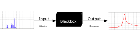
Mathematical modeling problems are often classified into black box or white box models, according to how much a priori information on the system is available. A black-box model is a system of which there is no a priori information available. A white-box model (also called glass box or clear box) is a system where all necessary information is available. Practically all systems are somewhere between the black-box and white-box models, so this concept is useful only as an intuitive guide for deciding which approach to take.
Usually it is preferable to use as much a priori information as possible to make the model more accurate. Therefore, the white-box models are usually considered easier, because if you have used the information correctly, then the model will behave correctly. Often the a priori information comes in forms of knowing the type of functions relating different variables. For example, if we make a model of how a medicine works in a human system, we know that usually the amount of medicine in the blood is an exponentially decaying function. But we are still left with several unknown parameters; how rapidly does the medicine amount decay, and what is the initial amount of medicine in blood? This example is therefore not a completely white-box model. These parameters have to be estimated through some means before one can use the model.
In black-box models one tries to estimate both the functional form of relations between variables and the numerical parameters in those functions. Using a priori information we could end up, for example, with a set of functions that probably could describe the system adequately. If there is no a priori information we would try to use functions as general as possible to cover all different models. An often used approach for black-box models are neural networks which usually do not make assumptions about incoming data. Alternatively the NARMAX (Nonlinear AutoRegressive Moving Average model with eXogenous inputs) algorithms which were developed as part of nonlinear system identification [3] can be used to select the model terms, determine the model structure, and estimate the unknown parameters in the presence of correlated and nonlinear noise. The advantage of NARMAX models compared to neural networks is that NARMAX produces models that can be written down and related to the underlying process, whereas neural networks produce an approximation that is opaque.
Subjective information
Sometimes it is useful to incorporate subjective information into a mathematical model. This can be done based on intuition, experience, or expert opinion, or based on convenience of mathematical form. Bayesian statistics provides a theoretical framework for incorporating such subjectivity into a rigorous analysis: we specify a prior probability distribution (which can be subjective), and then update this distribution based on empirical data.
An example of when such approach would be necessary is a situation in which an experimenter bends a coin slightly and tosses it once, recording whether it comes up heads, and is then given the task of predicting the probability that the next flip comes up heads. After bending the coin, the true probability that the coin will come up heads is unknown; so the experimenter would need to make a decision (perhaps by looking at the shape of the coin) about what prior distribution to use. Incorporation of such subjective information might be important to get an accurate estimate of the probability.
Complexity

In general, model complexity involves a trade-off between simplicity and accuracy of the model. Occam's razor is a principle particularly relevant to modeling; the essential idea being that among models with roughly equal predictive power, the simplest one is the most desirable. While added complexity usually improves the realism of a model, it can make the model difficult to understand and analyze, and can also pose computational problems, including numerical instability. Thomas Kuhn argues that as science progresses, explanations tend to become more complex before a paradigm shift offers radical simplification.
For example, when modeling the flight of an aircraft, we could embed each mechanical part of the aircraft into our model and would thus acquire an almost white-box model of the system. However, the computational cost of adding such a huge amount of detail would effectively inhibit the usage of such a model. Additionally, the uncertainty would increase due to an overly complex system, because each separate part induces some amount of variance into the model. It is therefore usually appropriate to make some approximations to reduce the model to a sensible size. Engineers often can accept some approximations in order to get a more robust and simple model. For example, Newton's classical mechanics is an approximated model of the real world. Still, Newton's model is quite sufficient for most ordinary-life situations, that is, as long as particle speeds are well below the speed of light, and we study macro-particles only.
Training
Any model which is not pure white-box contains some parameters that can be used to fit the model to the system it is intended to describe. If the modeling is done by a neural network or other machine learning, the optimization of parameters is called training, while the optimization of model hyperparameters is called tuning and often uses cross-validation. In more conventional modeling through explicitly given mathematical functions, parameters are often determined by curve fitting.
Model evaluation
A crucial part of the modeling process is the evaluation of whether or not a given mathematical model describes a system accurately. This question can be difficult to answer as it involves several different types of evaluation.
Fit to empirical data
Usually the easiest part of model evaluation is checking whether a model fits experimental measurements or other empirical data. In models with parameters, a common approach to test this fit is to split the data into two disjoint subsets: training data and verification data. The training data are used to estimate the model parameters. An accurate model will closely match the verification data even though these data were not used to set the model's parameters. This practice is referred to as cross-validation in statistics.
Defining a metric to measure distances between observed and predicted data is a useful tool of assessing model fit. In statistics, decision theory, and some economic models, a loss function plays a similar role.
While it is rather straightforward to test the appropriateness of parameters, it can be more difficult to test the validity of the general mathematical form of a model. In general, more mathematical tools have been developed to test the fit of statistical models than models involving differential equations. Tools from non-parametric statistics can sometimes be used to evaluate how well the data fit a known distribution or to come up with a general model that makes only minimal assumptions about the model's mathematical form.
Scope of the model
Assessing the scope of a model, that is, determining what situations the model is applicable to, can be less straightforward. If the model was constructed based on a set of data, one must determine for which systems or situations the known data is a "typical" set of data.
The question of whether the model describes well the properties of the system between data points is called interpolation, and the same question for events or data points outside the observed data is called extrapolation.
As an example of the typical limitations of the scope of a model, in evaluating Newtonian classical mechanics, we can note that Newton made his measurements without advanced equipment, so he could not measure properties of particles travelling at speeds close to the speed of light. Likewise, he did not measure the movements of molecules and other small particles, but macro particles only. It is then not surprising that his model does not extrapolate well into these domains, even though his model is quite sufficient for ordinary life physics.
Philosophical considerations
Many types of modeling implicitly involve claims about causality. This is usually (but not always) true of models involving differential equations. As the purpose of modeling is to increase our understanding of the world, the validity of a model rests not only on its fit to empirical observations, but also on its ability to extrapolate to situations or data beyond those originally described in the model. One can think of this as the differentiation between qualitative and quantitative predictions. One can also argue that a model is worthless unless it provides some insight which goes beyond what is already known from direct investigation of the phenomenon being studied.
An example of such criticism is the argument that the mathematical models of Optimal foraging theory do not offer insight that goes beyond the common-sense conclusions of evolution and other basic principles of ecology.[4]
Examples
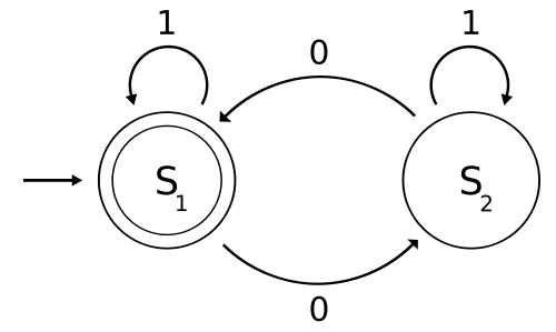
- One of the popular examples in computer science is the mathematical models of various machines, an example is the deterministic finite automaton which is defined as an abstract mathematical concept, but due to the deterministic nature of a DFA, it is implementable in hardware and software for solving various specific problems. For example, the following is a DFA M with a binary alphabet, which requires that the input contains an even number of 0s.
M = (Q, Σ, δ, q0, F) where
- Q = {S1, S2},
- Σ = {0, 1},
- q0 = S1,
- F = {S1}, and
- δ is defined by the following state transition table:
0 1 S1 S2 S1 S2 S1 S2
The state S1 represents that there has been an even number of 0s in the input so far, while S2 signifies an odd number. A 1 in the input does not change the state of the automaton. When the input ends, the state will show whether the input contained an even number of 0s or not. If the input did contain an even number of 0s, M will finish in state S1, an accepting state, so the input string will be accepted.
The language recognized by M is the regular language given by the regular expression 1*( 0 (1*) 0 (1*) )*, where "*" is the Kleene star, e.g., 1* denotes any non-negative number (possibly zero) of symbols "1".
- Many everyday activities carried out without a thought are uses of mathematical models. A geographical map projection of a region of the earth onto a small, plane surface is a model[5] which can be used for many purposes such as planning travel.
- Another simple activity is predicting the position of a vehicle from its initial position, direction and speed of travel, using the equation that distance traveled is the product of time and speed. This is known as dead reckoning when used more formally. Mathematical modeling in this way does not necessarily require formal mathematics; animals have been shown to use dead reckoning.[6][7]
- Population Growth. A simple (though approximate) model of population growth is the Malthusian growth model. A slightly more realistic and largely used population growth model is the logistic function, and its extensions.
- Individual-based cellular automata models of population growth
- Model of a particle in a potential-field. In this model we consider a particle as being a point of mass which describes a trajectory in space which is modeled by a function giving its coordinates in space as a function of time. The potential field is given by a function and the trajectory, that is a function , is the solution of the differential equation:


![-\frac{\mathrm{d}^2\mathbf{r}(t)}{\mathrm{d}t^2}m=\frac{\partial V[\mathbf{r}(t)]}{\partial x}\mathbf{\hat{x}}+\frac{\partial V[\mathbf{r}(t)]}{\partial y}\mathbf{\hat{y}}+\frac{\partial V[\mathbf{r}(t)]}{\partial z}\mathbf{\hat{z}},](../I/m/fd8f22ac8b8b4f56b4f541adcd524f759b5ed380.svg)
that can be written also as:
![m\frac{\mathrm{d}^2\mathbf{r}(t)}{\mathrm{d}t^2}=-\nabla V[\mathbf{r}(t)].](../I/m/fc987d59f3eb6aea08a9def1a21e4441af4456ea.svg)
- Note this model assumes the particle is a point mass, which is certainly known to be false in many cases in which we use this model; for example, as a model of planetary motion.
- Model of rational behavior for a consumer. In this model we assume a consumer faces a choice of n commodities labeled 1,2,...,n each with a market price p1, p2,..., pn. The consumer is assumed to have a cardinal utility function U (cardinal in the sense that it assigns numerical values to utilities), depending on the amounts of commodities x1, x2,..., xn consumed. The model further assumes that the consumer has a budget M which is used to purchase a vector x1, x2,..., xn in such a way as to maximize U(x1, x2,..., xn). The problem of rational behavior in this model then becomes an optimization problem, that is:
- subject to:
- This model has been used in general equilibrium theory, particularly to show existence and Pareto efficiency of economic equilibria. However, the fact that this particular formulation assigns numerical values to levels of satisfaction is the source of criticism (and even ridicule). However, it is not an essential ingredient of the theory and again this is an idealization.


- Neighbour-sensing model explains the mushroom formation from the initially chaotic fungal network.
- Computer science: models in Computer Networks, data models, surface model,...
- Mechanics: movement of rocket model,...
Modeling requires selecting and identifying relevant aspects of a situation in the real world.
See also
- Agent-based model
- Cliodynamics
- Computer simulation
- Conceptual model
- Decision engineering
- Grey box model
- Mathematical biology
- Mathematical diagram
- Mathematical psychology
- Mathematical sociology
- Model inversion
- Microscale and macroscale models
- Statistical Model
- System identification
- TK Solver - Rule Based Modeling
References
- ↑ Andreski, Stanislav (1972). Social Sciences as Sorcery. St. Martin’s Press. ISBN 0-14-021816-5.
- ↑ Truesdell, Clifford (1984). An Idiot’s Fugitive Essays on Science. Springer. pp. 121–7. ISBN 3-540-90703-3.
- ↑ Billings S.A. (2013), Nonlinear System Identification: NARMAX Methods in the Time, Frequency, and Spatio-Temporal Domains, Wiley.
- ↑ Pyke, G. H. (1984). "Optimal Foraging Theory: A Critical Review". Annual Review of Ecology and Systematics. 15: 523–575. doi:10.1146/annurev.es.15.110184.002515.
- ↑ landinfo.com, definition of map projection
- ↑ Gallistel (1990). The Organization of Learning. Cambridge: The MIT Press. ISBN 0-262-07113-4.
- ↑ Whishaw, I. Q.; Hines, D. J.; Wallace, D. G. (2001). "Dead reckoning (path integration) requires the hippocampal formation: Evidence from spontaneous exploration and spatial learning tasks in light (allothetic) and dark (idiothetic) tests". Behavioural Brain Research. 127 (1–2): 49–69. doi:10.1016/S0166-4328(01)00359-X. PMID 11718884.
Further reading
Books
- Aris, Rutherford [ 1978 ] ( 1994 ). Mathematical Modelling Techniques, New York: Dover. ISBN 0-486-68131-9
- Bender, E.A. [ 1978 ] ( 2000 ). An Introduction to Mathematical Modeling, New York: Dover. ISBN 0-486-41180-X
- Gershenfeld, N. (1998) The Nature of Mathematical Modeling, Cambridge University Press ISBN 0-521-57095-6 .
- Lin, C.C. & Segel, L.A. ( 1988 ). Mathematics Applied to Deterministic Problems in the Natural Sciences, Philadelphia: SIAM. ISBN 0-89871-229-7
Specific applications
- Korotayev A., Malkov A., Khaltourina D. (2006). Introduction to Social Macrodynamics: Compact Macromodels of the World System Growth. Moscow: Editorial URSS ISBN 5-484-00414-4 .
- Peierls, R. (1980). "Model-making in physics". Contemporary Physics. 21: 3–17. Bibcode:1980ConPh..21....3P. doi:10.1080/00107518008210938.
- An Introduction to Infectious Disease Modelling by Emilia Vynnycky and Richard G White.
External links
- General reference
- Patrone, F. Introduction to modeling via differential equations, with critical remarks.
- Plus teacher and student package: Mathematical Modelling. Brings together all articles on mathematical modeling from Plus Magazine, the online mathematics magazine produced by the Millennium Mathematics Project at the University of Cambridge.
- Philosophical
- Frigg, R. and S. Hartmann, Models in Science, in: The Stanford Encyclopedia of Philosophy, (Spring 2006 Edition)
- Griffiths, E. C. (2010) What is a model?