Lookup table
In computer science, a lookup table is an array that replaces runtime computation with a simpler array indexing operation. The savings in terms of processing time can be significant, since retrieving a value from memory is often faster than undergoing an "expensive" computation or input/output operation.[1] The tables may be precalculated and stored in static program storage, calculated (or "pre-fetched") as part of a program's initialization phase (memoization), or even stored in hardware in application-specific platforms. Lookup tables are also used extensively to validate input values by matching against a list of valid (or invalid) items in an array and, in some programming languages, may include pointer functions (or offsets to labels) to process the matching input. FPGAs also make extensive use of reconfigurable, hardware-implemented, lookup tables to provide programmable hardware functionality.
History
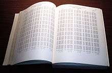
Before the advent of computers, lookup tables of values were used to speed up hand calculations of complex functions, such as in trigonometry, logarithms, and statistical density functions.[2]
In ancient (499 CE) India, Aryabhata created one of the first sine tables, which he encoded in a Sanskrit-letter-based number system. In 493 A.D., Victorius of Aquitaine wrote a 98-column multiplication table which gave (in Roman numerals) the product of every number from 2 to 50 times and the rows were "a list of numbers starting with one thousand, descending by hundreds to one hundred, then descending by tens to ten, then by ones to one, and then the fractions down to 1/144"[3] Modern school children are often taught to memorize "times tables" to avoid calculations of the most commonly used numbers (up to 9 x 9 or 12 x 12).
Early in the history of computers, input/output operations were particularly slow – even in comparison to processor speeds of the time. It made sense to reduce expensive read operations by a form of manual caching by creating either static lookup tables (embedded in the program) or dynamic prefetched arrays to contain only the most commonly occurring data items. Despite the introduction of systemwide caching that now automates this process, application level lookup tables can still improve performance for data items that rarely, if ever, change.
Lookup tables were one of the earliest functionalities implemented in computer spreadsheets, with the initial version of VisiCalc (1979) including a LOOKUP function among its original 20 functions.[4] This has been followed by subsequent spreadsheets, such as Microsoft Excel, and complemented by specialized VLOOKUP and HLOOKUP functions to simplify lookup in a vertical or horizontal table.
Examples
Simple lookup in an array, an associative array or a linked list (unsorted list)
This is known as a linear search or brute-force search, each element being checked for equality in turn and the associated value, if any, used as a result of the search. This is often the slowest search method unless frequently occurring values occur early in the list. For a one-dimensional array or linked list, the lookup is usually to determine whether or not there is a match with an 'input' data value.
Binary search in an array or an associative array (sorted list)
An example of a "divide and conquer algorithm", binary search involves each element being found by determining which half of the table a match may be found in and repeating until either success or failure. This is only possible if the list is sorted but gives good performance even if the list is lengthy.
Trivial hash function
For a trivial hash function lookup, the unsigned raw data value is used directly as an index to a one-dimensional table to extract a result. For small ranges, this can be amongst the fastest lookup, even exceeding binary search speed with zero branches and executing in constant time.
Counting bits in a series of bytes
One discrete problem that is expensive to solve on many computers, is that of counting the number of bits which are set to 1 in a (binary) number, sometimes called the population function. For example, the decimal number "37" is "00100101" in binary, so it contains three bits that are set to binary "1".
A simple example of C code, designed to count the 1 bits in a int, might look like this:
int count_ones(unsigned int x) {
    int result = 0;
    while (x != 0)
        result++, x = x & (x-1);
    return result;
}
This apparently simple algorithm can take potentially hundreds of cycles even on a modern architecture, because it makes many branches in the loop - and branching is slow. This can be ameliorated using loop unrolling and some other compiler optimizations. There is however a simple and much faster algorithmic solution - using a trivial hash function table lookup.
Simply construct a static table, bits_set, with 256 entries giving the number of one bits set in each possible byte value (e.g. 0x00 = 0, 0x01 = 1, 0x02 = 1, and so on). Then use this table to find the number of ones in each byte of the integer using a trivial hash function lookup on each byte in turn, and sum them. This requires no branches, and just four indexed memory accesses, considerably faster than the earlier code.
 /* Pseudocode of the lookup table 'uint32_t bits_set[256]' */
 /*                    0b00, 0b01, 0b10, 0b11, 0b100, 0b101, ... */
 int bits_set[256] = {    0,    1,    1,    2,     1,     2, // 200+ more entries

 /* (this code assumes that 'int' is an unsigned 32-bits wide integer) */
 int count_ones(unsigned int x) {
    return bits_set[ x        & 255] + bits_set[(x >>  8) & 255]
         + bits_set[(x >> 16) & 255] + bits_set[(x >> 24) & 255];
 }
The above source can be improved easily, (avoiding AND'ing, and shifting) by 'recasting' 'x' as a 4 byte unsigned char array and, preferably, coded in-line as a single statement instead of being a function. Note that even this simple algorithm can be too slow now, because the original code might run faster from the cache of modern processors, and (large) lookup tables do not fit well in caches and can cause a slower access to memory (in addition, in the above example, it requires computing addresses within a table, to perform the four lookups needed).
Lookup tables in image processing
In data analysis applications, such as image processing, a lookup table (LUT) is used to transform the input data into a more desirable output format. For example, a grayscale picture of the planet Saturn will be transformed into a color image to emphasize the differences in its rings.
A classic example of reducing run-time computations using lookup tables is to obtain the result of a trigonometry calculation, such as the sine of a value. Calculating trigonometric functions can substantially slow a computing application. The same application can finish much sooner when it first precalculates the sine of a number of values, for example for each whole number of degrees (The table can be defined as static variables at compile time, reducing repeated run time costs). When the program requires the sine of a value, it can use the lookup table to retrieve the closest sine value from a memory address, and may also take the step of interpolating to the sine of the desired value, instead of calculating by mathematical formula. Lookup tables are thus used by mathematics co-processors in computer systems. An error in a lookup table was responsible for Intel's infamous floating-point divide bug.
Functions of a single variable (such as sine and cosine) may be implemented by a simple array. Functions involving two or more variables require multidimensional array indexing techniques. The latter case may thus employ a two-dimensional array of power[x][y] to replace a function to calculate xy for a limited range of x and y values. Functions that have more than one result may be implemented with lookup tables that are arrays of structures.
As mentioned, there are intermediate solutions that use tables in combination with a small amount of computation, often using interpolation. Pre-calculation combined with interpolation can produce higher accuracy for values that fall between two precomputed values. This technique requires slightly more time to be performed but can greatly enhance accuracy in applications that require the higher accuracy. Depending on the values being precomputed, pre-computation with interpolation can also be used to shrink the lookup table size while maintaining accuracy.
In image processing, lookup tables are often called LUTs (or 3DLUT), and give an output value for each of a range of index values. One common LUT, called the colormap or palette, is used to determine the colors and intensity values with which a particular image will be displayed. In computed tomography, "windowing" refers to a related concept for determining how to display the intensity of measured radiation.
While often effective, employing a lookup table may nevertheless result in a severe penalty if the computation that the LUT replaces is relatively simple. Memory retrieval time and the complexity of memory requirements can increase application operation time and system complexity relative to what would be required by straight formula computation. The possibility of polluting the cache may also become a problem. Table accesses for large tables will almost certainly cause a cache miss. This phenomenon is increasingly becoming an issue as processors outpace memory. A similar issue appears in rematerialization, a compiler optimization. In some environments, such as the Java programming language, table lookups can be even more expensive due to mandatory bounds-checking involving an additional comparison and branch for each lookup.
There are two fundamental limitations on when it is possible to construct a lookup table for a required operation. One is the amount of memory that is available: one cannot construct a lookup table larger than the space available for the table, although it is possible to construct disk-based lookup tables at the expense of lookup time. The other is the time required to compute the table values in the first instance; although this usually needs to be done only once, if it takes a prohibitively long time, it may make the use of a lookup table an inappropriate solution. As previously stated however, tables can be statically defined in many cases.
Computing sines
Most computers, which only perform basic arithmetic operations, cannot directly calculate the sine of a given value. Instead, they use the CORDIC algorithm or a complex formula such as the following Taylor series to compute the value of sine to a high degree of precision:
- (for x close to 0)

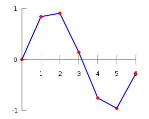
However, this can be expensive to compute, especially on slow processors, and there are many applications, particularly in traditional computer graphics, that need to compute many thousands of sine values every second. A common solution is to initially compute the sine of many evenly distributed values, and then to find the sine of x we choose the sine of the value closest to x. This will be close to the correct value because sine is a continuous function with a bounded rate of change. For example:
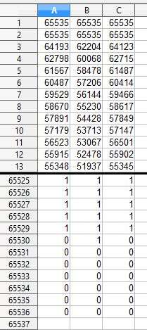
 real array sine_table[-1000..1000]
 for x from -1000 to 1000
     sine_table[x] := sine(pi * x / 1000)
 function lookup_sine(x)
     return sine_table[round(1000 * x / pi)]
Unfortunately, the table requires quite a bit of space: if IEEE double-precision floating-point numbers are used, over 16,000 bytes would be required. We can use fewer samples, but then our precision will significantly worsen. One good solution is linear interpolation, which draws a line between the two points in the table on either side of the value and locates the answer on that line. This is still quick to compute, and much more accurate for smooth functions such as the sine function. Here is our example using linear interpolation:
 function lookup_sine(x)
     x1 := floor(x*1000/pi)
     y1 := sine_table[x1]
     y2 := sine_table[x1+1]
     return y1 + (y2-y1)*(x*1000/pi-x1)
Another solution that uses a quarter of the space but takes a bit longer to compute would be to take into account the relationships between sine and cosine along with their symmetry rules. In this case, the lookup table is calculated by using the sine function for the first quadrant (i.e. sin(0..pi/2)). When we need a value, we assign a variable to be the angle wrapped to the first quadrant. We then wrap the angle to the four quadrants (not needed if values are always between 0 and 2*pi) and return the correct value (i.e. first quadrant is a straight return, second quadrant is read from pi/2-x, third and fourth are negatives of the first and second respectively). For cosine, we only have to return the angle shifted by pi/2 (i.e. x+pi/2). For tangent, we divide the sine by the cosine (divide-by-zero handling may be needed depending on implementation):
 function init_sine()
     for x from 0 to (360/4)+1
         sine_table[x] := sine(2*pi * x / 360)

 function lookup_sine(x)
     x  = wrap x from 0 to 360
     y := mod (x, 90)

     if (x <  90) return  sine_table[   y]
     if (x < 180) return  sine_table[90-y]
     if (x < 270) return -sine_table[   y]
                  return -sine_table[90-y]

 function lookup_cosine(x)
     return lookup_sine(x + 90)

 function lookup_tan(x)
     return (lookup_sine(x) / lookup_cosine(x))
When using interpolation, the size of the lookup table can be reduced by using nonuniform sampling, which means that where the function is close to straight, we use few sample points, while where it changes value quickly we use more sample points to keep the approximation close to the real curve. For more information, see interpolation.
Other usage of lookup tables
Caches
Storage caches (including disk caches for files, or processor caches for either code or data) work also like a lookup table. The table is built with very fast memory instead of being stored on slower external memory, and maintains two pieces of data for a subrange of bits composing an external memory (or disk) address (notably the lowest bits of any possible external address):
- one piece (the tag) contains the value of the remaining bits of the address; if these bits match with those from the memory address to read or write, then the other piece contains the cached value for this address.
- the other piece maintains the data associated to that address.
A single (fast) lookup is performed to read the tag in the lookup table at the index specified by the lowest bits of the desired external storage address, and to determine if the memory address is hit by the cache. When a hit is found, no access to external memory is needed (except for write operations, where the cached value may need to be updated asynchronously to the slower memory after some time, or if the position in the cache must be replaced to cache another address).
Hardware LUTs
In digital logic, a lookup table can be implemented with a multiplexer whose select lines are driven by the address signal and whose inputs are the values of the elements contained in the array. These values can either be hard-wired, as in an ASIC which purpose is specific to a function, or provided by D latches which allow for configurable values.
An n-bit LUT can encode any n-input boolean function by storing the truth table of the function in the LUT. This is an efficient way of encoding Boolean logic functions, and LUTs with 4-6 bits of input are in fact the key component of modern field-programmable gate arrays (FPGAs) which provide reconfigurable hardware logic capabilities.
See also
- Associative array
- Branch table
- Gal's accurate tables
- Memoization
- Memory bound function
- Shift register lookup table
- Palette and Colour Look-Up Table – for the usage in computer graphics
- 3D LUT – usage in film
References
- ↑ http://pmcnamee.net/c++-memoization.html
- ↑ Campbell-Kelly, Martin; Croarken, Mary; Robson, Eleanor, eds. (October 2, 2003) [2003]. The History of Mathematical Tables From Sumer to Spreadsheets (1st ed.). New York, USA. ISBN 978-0-19-850841-0.
- ↑ Maher, David. W. J. and John F. Makowski. "Literary Evidence for Roman Arithmetic With Fractions", 'Classical Philology' (2001) Vol. 96 No. 4 (2001) pp. 376–399. (See page p.383.)
- ↑ Bill Jelen: “From 1979 – VisiCalc and LOOKUP”!, by MrExcel East, March 31, 2012
External links
- Fast table lookup using input character as index for branch table
- Art of Assembly: Calculation via Table Lookups
- "Bit Twiddling Hacks" (includes lookup tables) By Sean Eron Anderson of Stanford university
- Memoization in C++ by Paul McNamee, Johns Hopkins University showing savings
- "The Quest for an Accelerated Population Count" by Henry S. Warren, Jr.