Logit

This article discusses the binary logit function only. See discrete choice for a discussion of multinomial logit, conditional logit, nested logit, mixed logit, exploded logit, and ordered logit. For the basic regression technique that uses the logit function, see logistic regression.

Plot of logit(p) in the domain of 0 to 1, where the base of logarithm is e

The logit (/ˈloʊdʒɪt/ LOH-jit) function is the inverse of the sigmoidal "logistic" function or logistic transform used in mathematics, especially in statistics. When the function's parameter represents a probability $p$ , the logit function gives the log-odds, or the logarithm of the odds $p /(1 - p)$ .^[1]

Definition

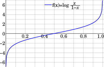
The logit of a number p between 0 and 1 is given by the formula:

\operatorname {logit} (p)=\log \left({\frac {p}{1-p}}\right)=\log(p)-\log(1-p)=-\log \left({\frac {1}{p}}-1\right).\!\,

The base of the logarithm function used is of little importance in the present article, as long as it is greater than 1, but the natural logarithm with base e is the one most often used. The choice of base corresponds to the choice of logarithmic unit for the value: base 2 corresponds to a bit, base e to a nat, and base 10 to a ban (dit, hartley); these units are particularly used in information-theoretic interpretations. For each choice of base, the logit function takes values between negative and positive infinity.

The "logistic" function of any number $\alpha$ is given by the inverse-logit:

\operatorname {logit} ^{-1}(\alpha )=\operatorname {logistic} (\alpha )={\frac {1}{1+\operatorname {exp} (-\alpha )}}={\frac {\operatorname {exp} (\alpha )}{\operatorname {exp} (\alpha )+1}}

If p is a probability, then p/(1 − p) is the corresponding odds; the logit of the probability is the logarithm of the odds. Similarly, the difference between the logits of two probabilities is the logarithm of the odds ratio (R), thus providing a shorthand for writing the correct combination of odds ratios only by adding and subtracting:

\operatorname {log} (R)=\log \left({\frac {{p_{1}}/(1-p_{1})}{{p_{2}}/(1-p_{2})}}\right)=\log \left({\frac {p_{1}}{1-p_{1}}}\right)-\log \left({\frac {p_{2}}{1-p_{2}}}\right)=\operatorname {logit} (p_{1})-\operatorname {logit} (p_{2}).\!\,

History

Log odds was used extensively by Charles Sanders Peirce (late 19th century).^[2] The logit model was introduced by Joseph Berkson in 1944, who coined the term. The term was borrowed by analogy from the very similar probit model developed by Chester Ittner Bliss in 1934.^[3] G. A. Barnard in 1949 coined the commonly used term log-odds;^[4] the log-odds of an event is the logit of the probability of the event.^[5]

Uses and properties

The logit in logistic regression is a special case of a link function in a generalized linear model: it is the canonical link function for the Bernoulli distribution.
The logit function is the negative of the derivative of the binary entropy function.
The logit is also central to the probabilistic Rasch model for measurement, which has applications in psychological and educational assessment, among other areas.
The inverse-logit function (i.e., the logistic function) is also sometimes referred to as the expit function.^[6]
In plant disease epidemiology the logit is used to fit the data to a logistic model. With the Gompertz and Monomolecular models all three are known as Richards family models.

Comparison with probit

Comparison of the logit function with a scaled probit (i.e. the inverse CDF of the normal distribution), comparing

\operatorname {logit} (x)

vs.

\Phi ^{-1}(x)/{\sqrt {\frac {\pi }{8}}}

, which makes the slopes the same at the y-origin.

Closely related to the logit function (and logit model) are the probit function and probit model. The logit and probit are both sigmoid functions with a domain between 0 and 1, which makes them both quantile functions—i.e., inverses of the cumulative distribution function (CDF) of a probability distribution. In fact, the logit is the quantile function of the logistic distribution, while the probit is the quantile function of the normal distribution. The probit function is denoted $\Phi ^{-1}(x)$ , where $\Phi (x)$ is the CDF of the normal distribution, as just mentioned:

\Phi (x)=\int _{-\infty }^{x}{\frac {1}{\sqrt {2\pi }}}e^{-{\frac {z^{2}}{2}}}\operatorname {d} \!z

As shown in the graph, the logit and probit functions are extremely similar, particularly when the probit function is scaled so that its slope at y=0 matches the slope of the logit. As a result, probit models are sometimes used in place of logit models because for certain applications (e.g., in Bayesian statistics) the implementation is easier.

References

↑ "LOG ODDS RATIO". nist.gov.
↑ Stigler, Stephen M. (1986). The history of statistics : the measurement of uncertainty before 1900. Cambridge, Mass: Belknap Press of Harvard University Press. ISBN 0-674-40340-1.
1 2 J. S. Cramer (2003). "The origins and development of the logit model" (PDF). Cambridge UP.
↑ Hilbe, Joseph M. (2009), Logistic Regression Models, CRC Press, p. 3, ISBN 9781420075779 .
↑ Cramer, J. S. (2003), Logit Models from Economics and Other Fields, Cambridge University Press, p. 13, ISBN 9781139438193 .
↑ http://www.stat.ucl.ac.be/ISdidactique/Rhelp/library/msm/html/expit.html