List of formulas in Riemannian geometry
This is a list of formulas encountered in Riemannian geometry.
Christoffel symbols, covariant derivative
In a smooth coordinate chart, the Christoffel symbols of the first kind are given by

and the Christoffel symbols of the second kind by
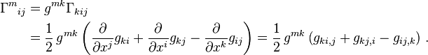
Here  is the inverse matrix to the metric tensor
  . In other words,

and thus
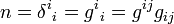
is the dimension of the manifold.
Christoffel symbols satisfy the symmetry relations
 or, respectively,
  ,
,
the second of which is equivalent to the torsion-freeness of the Levi-Civita connection.
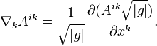
The contracting relations on the Christoffel symbols are given by
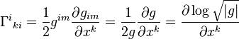
and
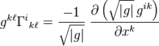
where |g| is the absolute value of the determinant of the metric tensor  . These are useful when dealing with divergences and Laplacians (see below).
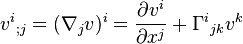
The covariant derivative of a vector field with components  is given by:
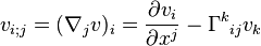
and similarly the covariant derivative of a  -tensor field with components
  is given by:
For a  -tensor field with components
  this becomes

and likewise for tensors with more indices.
The covariant derivative of a function (scalar)  is just its usual differential:

Because the Levi-Civita connection is metric-compatible, the covariant derivatives of metrics vanish,
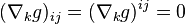
as well as the covariant derivatives of the metric's determinant (and volume element)

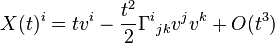
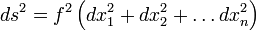
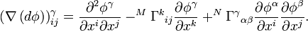
The geodesic  starting at the origin with initial speed has Taylor expansion in the chart:
Curvature tensors
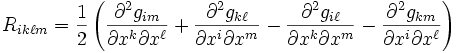
Riemann curvature tensor
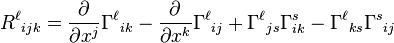
If one defines the curvature operator as ![R(U,V)W=\nabla_U \nabla_V W - \nabla_V \nabla_U W -\nabla_{[U,V]}W](../I/m/afd19f70d73e2f9ccd4957db1cf961cd.png) and the coordinate components of the
and the coordinate components of the  -Riemann curvature tensor by
 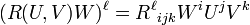 , then these components are given by:
Lowering indices with  one gets

The symmetries of the tensor are
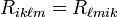 and
and 
That is, it is symmetric in the exchange of the first and last pair of indices, and antisymmetric in the flipping of a pair.
The cyclic permutation sum (sometimes called first Bianchi identity) is

The (second) Bianchi identity is

that is,

which amounts to a cyclic permutation sum of the last three indices, leaving the first two fixed.
Ricci and scalar curvatures
Ricci and scalar curvatures are contractions of the Riemann tensor. They simplify the Riemann tensor, but contain less information.
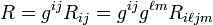
The Ricci curvature tensor is essentially the unique nontrivial way of contracting the Riemann tensor:

The Ricci tensor  is symmetric.
By the contracting relations on the Christoffel symbols, we have

The scalar curvature is the trace of the Ricci curvature,
 .
.
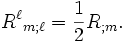
The "gradient" of the scalar curvature follows from the Bianchi identity (proof):
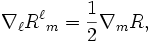
that is,
Einstein tensor
The Einstein tensor Gab is defined in terms of the Ricci tensor Rab and the Ricci scalar R,
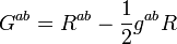
where g is the metric tensor.
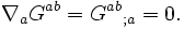
The Einstein tensor is symmetric, with a vanishing divergence (proof) which is due to the Bianchi identity:
Weyl tensor
The Weyl tensor is given by

where  denotes the dimension of the Riemannian manifold.
The Weyl tensor satisfies the first (algebraic) Bianchi identity:

The Weyl tensor is a symmetric product of alternating 2-forms,

just like the Riemann tensor. Moreover, taking the trace over any two indices gives zero,

The Weyl tensor vanishes ( ) if and only if a manifold
  of dimension
  is locally conformally flat. In other words, can be covered by coordinate systems in which the metric
  satisfies
This is essentially because  is invariant under conformal changes.
Gradient, divergence, Laplace–Beltrami operator
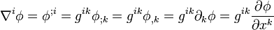
The gradient of a function is obtained by raising the index of the differential  , whose components are given by:
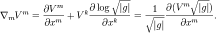
The divergence of a vector field with components  is
is
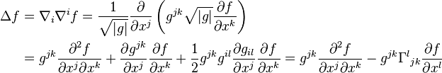
The Laplace–Beltrami operator acting on a function  is given by the divergence of the gradient:
The divergence of an antisymmetric tensor field of type simplifies to
The Hessian of a map  is given by
Kulkarni–Nomizu product
The Kulkarni–Nomizu product is an important tool for constructing new tensors from existing tensors on a Riemannian manifold. Let  and
and  be symmetric covariant 2-tensors. In coordinates,

Then we can multiply these in a sense to get a new covariant 4-tensor, which is often denoted  . The defining formula is

Clearly, the product satisfies

In an inertial frame
An orthonormal inertial frame is a coordinate chart such that, at the origin, one has the relations  and
and  (but these may not hold at other points in the frame). These coordinates are also called normal coordinates.
In such a frame, the expression for several operators is simpler. Note that the formulae given below are valid at the origin of the frame only.
(but these may not hold at other points in the frame). These coordinates are also called normal coordinates.
In such a frame, the expression for several operators is simpler. Note that the formulae given below are valid at the origin of the frame only.

Under a conformal change
Let  be a Riemannian metric on a smooth manifold , and
  a smooth real-valued function on . Then

is also a Riemannian metric on . We say that  is conformal to . Evidently, conformality of metrics is an equivalence relation. Here are some formulas for conformal changes in tensors associated with the metric. (Quantities marked with a tilde will be associated with , while those unmarked with such will be associated with .)


Note that the difference between the Christoffel symbols of two different metrics always form the components of a tensor.
We can also write this in a coordinate-free manner:
 ,
,
(where  is the conformal map, i.e.:
  , and
, and  are vector fields.)

Here  is the Riemannian volume element.
![\tilde R_{ijkl} = e^{2\varphi}\left( R_{ijkl} - \left[ g {~\wedge\!\!\!\!\!\!\bigcirc~} \left( \nabla\partial\varphi - \partial\varphi\partial\varphi + \frac{1}{2}\|\nabla\varphi\|^2g \right)\right]_{ijkl} \right)](../I/m/c53975cc1a42c0a1431e138a18471644.png)
Here  is the Kulkarni–Nomizu product defined earlier in this article. The symbol
  denotes partial derivative, while
  denotes covariant derivative.
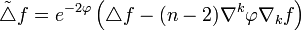
![\tilde R_{ij} = R_{ij} - (n-2)\left[ \nabla_i\partial_j \varphi - (\partial_i \varphi)(\partial_j \varphi) \right] + \left( \triangle \varphi - (n-2)\|\nabla \varphi\|^2 \right)g_{ij}](../I/m/667ef988dd8b776aecb1ac9989d8b876.png)
Beware that here the Laplacian  is minus the trace of the Hessian on functions,
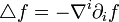
Thus the operator  is elliptic because the metric is Riemannian.

If the dimension  , then this simplifies to
![\tilde R = e^{-2\varphi}\left[R + \frac{4(n-1)}{(n-2)}e^{-(n-2)\varphi/2}\triangle\left( e^{(n-2)\varphi/2} \right) \right]](../I/m/208505f0b38e8b724d0a71d0de55e156.png)

We see that the (3,1) Weyl tensor is invariant under conformal changes.
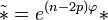
Let  be a differential
  -form. Let
  be the Hodge star, and
  the codifferential. Under a conformal change, these satisfy
 = e^{-2\varphi}\left[ \delta\omega - (n-2p)\omega\left(\nabla\varphi, v_1, v_2, \ldots , v_{p-1}\right) \right]](../I/m/0bf855bfff99e0d0f93dee4ab3abd842.png)