Laplace transform

"ℒ" redirects here. For the Lagrangian, see Lagrangian mechanics.

In mathematics the Laplace transform is an integral transform named after its discoverer Pierre-Simon Laplace (/ləˈplɑːs/). It takes a function of a positive real variable $t$ (often time) to a function of a complex variable $s$ (frequency).

The Laplace transform is very similar to the Fourier transform. While the Fourier transform of a function is a complex function of a real variable (frequency), the Laplace transform of a function is a complex function of a complex variable. Laplace transforms are usually restricted to functions of $t$ with $t > 0$ . A consequence of this restriction is that the Laplace transform of a function is a holomorphic function of the variable $s$ . Unlike the Fourier transform, the Laplace transform of a distribution is generally a well-behaved function. Also techniques of complex variables can be used directly to study Laplace transforms. As a holomorphic function, the Laplace transform has a power series representation. This power series expresses a function as a linear superposition of moments of the function. This perspective has applications in probability theory.

The Laplace transform is invertible on a large class of functions. The inverse Laplace transform takes a function of a complex variable s (often frequency) and yields a function of a real variable t (time). Given a simple mathematical or functional description of an input or output to a system, the Laplace transform provides an alternative functional description that often simplifies the process of analyzing the behavior of the system, or in synthesizing a new system based on a set of specifications.^[1] So, for example, Laplace transformation from the time domain to the frequency domain transforms differential equations into algebraic equations and convolution into multiplication. It has many applications in the sciences and technology.

History

The Laplace transform is named after mathematician and astronomer Pierre-Simon Laplace, who used a similar transform (now called the z-transform) in his work on probability theory.^[2] The current widespread use of the transform (mainly in engineering) came about during and soon after World War II ^[3] although it had been used in the 19th century by Abel, Lerch, Heaviside, and Bromwich.

The early history of methods having some similarity to Laplace transform is as follows. From 1744, Leonhard Euler investigated integrals of the form

z=\int X(x)e^{ax}\,dx\quad {\text{ and }}\quad z=\int X(x)x^{A}\,dx

as solutions of differential equations but did not pursue the matter very far.^[4]

Joseph Louis Lagrange was an admirer of Euler and, in his work on integrating probability density functions, investigated expressions of the form

\int X(x)e^{-ax}a^{x}\,dx,

which some modern historians have interpreted within modern Laplace transform theory.^[5]^[6]

These types of integrals seem first to have attracted Laplace's attention in 1782 where he was following in the spirit of Euler in using the integrals themselves as solutions of equations.^[7] However, in 1785, Laplace took the critical step forward when, rather than just looking for a solution in the form of an integral, he started to apply the transforms in the sense that was later to become popular. He used an integral of the form

\int x^{s}\phi (x)\,dx,

akin to a Mellin transform, to transform the whole of a difference equation, in order to look for solutions of the transformed equation. He then went on to apply the Laplace transform in the same way and started to derive some of its properties, beginning to appreciate its potential power.^[8]

Laplace also recognised that Joseph Fourier's method of Fourier series for solving the diffusion equation could only apply to a limited region of space because those solutions were periodic. In 1809, Laplace applied his transform to find solutions that diffused indefinitely in space.^[9]

Formal definition

The Laplace transform is a frequency-domain approach for continuous time signals irrespective of whether the system is stable or unstable. The Laplace transform of a function $f (t)$ , defined for all real numbers $t \geq 0$ , is the function $F (s)$ , which is a unilateral transform defined by

F(s)=\int _{0}^{\infty }e^{-st}f(t)\,dt

where s is a complex number frequency parameter

s=\sigma +i\omega

, with real numbers

σ

and

ω

Other notations for the Laplace transform include $L {f}$ , or alternatively $L {f (t)}$ instead of $F$ .

The meaning of the integral depends on types of functions of interest. A necessary condition for existence of the integral is that $f$ must be locally integrable on $[0, \infty)$ . For locally integrable functions that decay at infinity or are of exponential type, the integral can be understood to be a (proper) Lebesgue integral. However, for many applications it is necessary to regard it to be a conditionally convergent improper integral at $\infty$ . Still more generally, the integral can be understood in a weak sense, and this is dealt with below.

One can define the Laplace transform of a finite Borel measure $μ$ by the Lebesgue integral^[10]

{\mathcal {L}}\{\mu \}(s)=\int _{[0,\infty )}e^{-st}\,d\mu (t).

An important special case is where $μ$ is a probability measure, for example, the Dirac delta function. In operational calculus, the Laplace transform of a measure is often treated as though the measure came from a probability density function $f$ . In that case, to avoid potential confusion, one often writes

{\mathcal {L}}\{f\}(s)=\int _{0^{-}}^{\infty }e^{-st}f(t)\,dt,

where the lower limit of $0 -$ is shorthand notation for

\lim _{\varepsilon \downarrow 0}\int _{-\varepsilon }^{\infty }.

This limit emphasizes that any point mass located at $0$ is entirely captured by the Laplace transform. Although with the Lebesgue integral, it is not necessary to take such a limit, it does appear more naturally in connection with the Laplace–Stieltjes transform.

Probability theory

In pure and applied probability, the Laplace transform is defined as an expected value. If $X$ is a random variable with probability density function $f$ , then the Laplace transform of $f$ is given by the expectation

{\mathcal {L}}\{f\}(s)=E\!\left[e^{-sX}\right]\!.

By abuse of language, this is referred to as the Laplace transform of the random variable $X$ itself. Replacing $s$ by $- t$ gives the moment generating function of $X$ . The Laplace transform has applications throughout probability theory, including first passage times of stochastic processes such as Markov chains, and renewal theory.

Of particular use is the ability to recover the cumulative distribution function of a continuous random variable $X$ by means of the Laplace transform as follows^[11]

F_{X}(x)={\mathcal {L}}^{-1}\!\left\{{\frac {1}{s}}E\left[e^{-sX}\right]\right\}\!(x)={\mathcal {L}}^{-1}\!\left\{{\frac {1}{s}}{\mathcal {L}}\{f\}(s)\right\}\!(x).

Bilateral Laplace transform

Main article: Two-sided Laplace transform

When one says "the Laplace transform" without qualification, the unilateral or one-sided transform is normally intended. The Laplace transform can be alternatively defined as the bilateral Laplace transform or two-sided Laplace transform by extending the limits of integration to be the entire real axis. If that is done the common unilateral transform simply becomes a special case of the bilateral transform where the definition of the function being transformed is multiplied by the Heaviside step function.

The bilateral Laplace transform is defined as follows,

{\mathcal {B}}\{f\}(s)=\int _{-\infty }^{\infty }e^{-st}f(t)\,dt.

Inverse Laplace transform

Main article: Inverse Laplace transform

Two integrable functions have the same Laplace transform only if they differ on a set of Lebesgue measure zero. This means that, on the range of the transform, there is an inverse transform. In fact, besides integrable functions, the Laplace transform is a one-to-one mapping from one function space into another in many other function spaces as well, although there is usually no easy characterization of the range. Typical function spaces in which this is true include the spaces of bounded continuous functions, the space $L \infty (0, \infty)$ , or more generally tempered functions (that is, functions of at worst polynomial growth) on $(0, \infty)$ . The Laplace transform is also defined and injective for suitable spaces of tempered distributions.

In these cases, the image of the Laplace transform lives in a space of analytic functions in the region of convergence. The inverse Laplace transform is given by the following complex integral, which is known by various names (the Bromwich integral, the Fourier–Mellin integral, and Mellin's inverse formula):

f(t)={\mathcal {L}}^{-1}\{F\}(t)={\frac {1}{2\pi i}}\lim _{T\to \infty }\int _{\gamma -iT}^{\gamma +iT}e^{st}F(s)\,ds,

where $γ$ is a real number so that the contour path of integration is in the region of convergence of $F (s)$ . An alternative formula for the inverse Laplace transform is given by Post's inversion formula. The limit here is interpreted in the weak-* topology.

In practice, it is typically more convenient to decompose a Laplace transform into known transforms of functions obtained from a table, and construct the inverse by inspection.

Region of convergence

If $f$ is a locally integrable function (or more generally a Borel measure locally of bounded variation), then the Laplace transform $F (s)$ of $f$ converges provided that the limit

\lim _{R\to \infty }\int _{0}^{R}f(t)e^{-st}\,dt

exists.

The Laplace transform converges absolutely if the integral

\int _{0}^{\infty }\left|f(t)e^{-st}\right|\,dt

exists (as a proper Lebesgue integral). The Laplace transform is usually understood as conditionally convergent, meaning that it converges in the former instead of the latter sense.

The set of values for which $F (s)$ converges absolutely is either of the form $Re(s) > a$ or else $Re(s) \geq a$ , where $a$ is an extended real constant, $-\infty \leq a \leq \infty$ . (This follows from the dominated convergence theorem.) The constant $a$ is known as the abscissa of absolute convergence, and depends on the growth behavior of $f (t)$ .^[12] Analogously, the two-sided transform converges absolutely in a strip of the form $a < Re(s) < b$ , and possibly including the lines $Re(s) = a$ or $Re(s) = b$ .^[13] The subset of values of $s$ for which the Laplace transform converges absolutely is called the region of absolute convergence or the domain of absolute convergence. In the two-sided case, it is sometimes called the strip of absolute convergence. The Laplace transform is analytic in the region of absolute convergence.

Similarly, the set of values for which $F (s)$ converges (conditionally or absolutely) is known as the region of conditional convergence, or simply the region of convergence (ROC). If the Laplace transform converges (conditionally) at $s = s 0$ , then it automatically converges for all $s$ with $Re(s) > Re(s 0)$ . Therefore, the region of convergence is a half-plane of the form $Re(s) > a$ , possibly including some points of the boundary line $Re(s) = a$ .

In the region of convergence $Re(s) > Re(s 0)$ , the Laplace transform of $f$ can be expressed by integrating by parts as the integral

F(s)=(s-s_{0})\int _{0}^{\infty }e^{-(s-s_{0})t}\beta (t)\,dt,\quad \beta (u)=\int _{0}^{u}e^{-s_{0}t}f(t)\,dt.

That is, in the region of convergence $F (s)$ can effectively be expressed as the absolutely convergent Laplace transform of some other function. In particular, it is analytic.

There are several Paley–Wiener theorems concerning the relationship between the decay properties of $f$ and the properties of the Laplace transform within the region of convergence.

In engineering applications, a function corresponding to a linear time-invariant (LTI) system is stable if every bounded input produces a bounded output. This is equivalent to the absolute convergence of the Laplace transform of the impulse response function in the region $Re(s) \geq 0$ . As a result, LTI systems are stable provided the poles of the Laplace transform of the impulse response function have negative real part.

This ROC is used in knowing about the causality and stability of a system.

Properties and theorems

The Laplace transform has a number of properties that make it useful for analyzing linear dynamical systems. The most significant advantage is that differentiation and integration become multiplication and division, respectively, by $s$ (similarly to logarithms changing multiplication of numbers to addition of their logarithms).

Because of this property, the Laplace variable $s$ is also known as operator variable in the $L$ domain: either derivative operator or (for $s -1)$ integration operator. The transform turns integral equations and differential equations to polynomial equations, which are much easier to solve. Once solved, use of the inverse Laplace transform reverts to the time domain.

Given the functions $f (t)$ and $g (t)$ , and their respective Laplace transforms $F (s)$ and $G (s)$ ,

{\begin{aligned}f(t)&={\mathcal {L}}^{-1}\{F(s)\},\\g(t)&={\mathcal {L}}^{-1}\{G(s)\},\end{aligned}}

The following Table is a list of properties of unilateral Laplace transform:^[14]

Properties of the unilateral Laplace transform
	Time domain	$s$ domain	Comment
Linearity	$af(t)+bg(t)\$	$aF(s)+bG(s)\$	Can be proved using basic rules of integration.
Frequency-domain derivative	$tf(t)\$	$-F'(s)\$	$F'$ is the first derivative of $F$ .
Frequency-domain general derivative	$t^{n}f(t)\$	$(-1)^{n}F^{(n)}(s)\$	More general form, $n$ th derivative of $F (s)$ .
Derivative	$f'(t)\$	$sF(s)-f(0)\$	$f$ is assumed to be a differentiable function, and its derivative is assumed to be of exponential type. This can then be obtained by integration by parts
Second derivative	$f''(t)\$	$s^{2}F(s)-sf(0)-f'(0)\$	$f$ is assumed twice differentiable and the second derivative to be of exponential type. Follows by applying the Differentiation property to $f'(t)$ .
General derivative	$f^{(n)}(t)\$	$s^{n}F(s)-\sum _{k=1}^{n}s^{n-k}f^{(k-1)}(0)\$	$f$ is assumed to be $n$ -times differentiable, with $n$ th derivative of exponential type. Follows by mathematical induction.
Frequency-domain integration	${\frac {1}{t}}f(t)\$	$\int _{s}^{\infty }F(\sigma )\,d\sigma \$	This is deduced using the nature of frequency differentiation and conditional convergence.
Time-domain integration	$\int _{0}^{t}f(\tau )\,d\tau =(u*f)(t)$	${1 \over s}F(s)$	$u (t)$ is the Heaviside step function. Note that $(u * f)(t)$ is the convolution of $u (t)$ and $f (t)$ .
Frequency shifting	$e^{at}f(t)\$	$F(s-a)\$
Time shifting	$f(t-a)u(t-a)\$	$e^{-as}F(s)\$	$u (t)$ is the Heaviside step function
Time scaling	$f(at)$	${\frac {1}{a}}F\left({s \over a}\right)$	$a>0\$
Multiplication	$f(t)g(t)$	${\frac {1}{2\pi i}}\lim _{T\to \infty }\int _{c-iT}^{c+iT}F(\sigma )G(s-\sigma )\,d\sigma \$	The integration is done along the vertical line Re(σ) = c that lies entirely within the region of convergence of $F$ .^[15]
Convolution	$(f*g)(t)=\int _{0}^{t}f(\tau )g(t-\tau )\,d\tau$	$F(s)\cdot G(s)\$
Complex conjugation	$f^{*}(t)$	$F^{}(s^{})$
Cross-correlation	$f(t)\star g(t)$	$F^{}(-s^{})\cdot G(s)$
Periodic function	$f(t)$	${1 \over 1-e^{-Ts}}\int _{0}^{T}e^{-st}f(t)\,dt$	$f (t)$ is a periodic function of period $T$ so that $f (t) = f (t + T)$ , for all $t \geq 0$ . This is the result of the time shifting property and the geometric series.

Initial value theorem:

f(0^{+})=\lim _{s\to \infty }{sF(s)}.

Final value theorem:

f(\infty )=\lim _{s\to 0}{sF(s)}

, if all poles of sF(s) are in the left half-plane.

The final value theorem is useful because it gives the long-term behaviour without having to perform partial fraction decompositions or other difficult algebra. If

F (s)

has a pole in the right-hand plane or poles on the imaginary axis (e.g., if

f(t)=e^{t}

f(t)=\sin(t)

), the behaviour of this formula is undefined.

Relation to power series

The Laplace transform can be viewed as a continuous analogue of a power series. If $a (n)$ is a discrete function of a positive integer $n$ , then the power series associated to $a (n)$ is the series

\sum _{n=0}^{\infty }a(n)x^{n}

where $x$ is a real variable (see Z transform). Replacing summation over $n$ with integration over $t$ , a continuous version of the power series becomes

\int _{0}^{\infty }f(t)x^{t}\,dt

where the discrete function $a (n)$ is replaced by the continuous one $f (t)$ . (See Mellin transform below.)

Changing the base of the power from $x$ to $e$ gives

\int _{0}^{\infty }f(t)\left(e^{\ln {x}}\right)^{t}\,dt

For this to converge for, say, all bounded functions $f$ , it is necessary to require that $ln x < 0$ . Making the substitution $- s = ln x$ gives just the Laplace transform:

\int _{0}^{\infty }f(t)e^{-st}\,dt

In other words, the Laplace transform is a continuous analog of a power series in which the discrete parameter $n$ is replaced by the continuous parameter $t$ , and $x$ is replaced by $e - s$ .

Relation to moments

Main article: Moment generating function

The quantities

\mu _{n}=\int _{0}^{\infty }t^{n}f(t)\,dt

are the moments of the function $f$ . If the first $n$ moments of $f$ converge absolutely, then by repeated differentiation under the integral,

(-1)^{n}({\mathcal {L}}f)^{(n)}(0)=\mu _{n}.

This is of special significance in probability theory, where the moments of a random variable $X$ are given by the expectation values $\mu _{n}=E[X^{n}]$ . Then, the relation holds

\mu _{n}=(-1)^{n}{\frac {d^{n}}{ds^{n}}}E\left[e^{-sX}\right](0).

Proof of the Laplace transform of a function's derivative

It is often convenient to use the differentiation property of the Laplace transform to find the transform of a function's derivative. This can be derived from the basic expression for a Laplace transform as follows:

{\begin{aligned}{\mathcal {L}}\left\{f(t)\right\}&=\int _{0^{-}}^{\infty }e^{-st}f(t)\,dt\\&=\left[{\frac {f(t)e^{-st}}{-s}}\right]_{0^{-}}^{\infty }-\int _{0^{-}}^{\infty }{\frac {e^{-st}}{-s}}f'(t)\,dt\quad {\text{(by parts)}}\\&=\left[-{\frac {f(0^{-})}{-s}}\right]+{\frac {1}{s}}{\mathcal {L}}\left\{f'(t)\right\},\end{aligned}}

yielding

{\mathcal {L}}\left\{f'(t)\right\}=s\cdot {\mathcal {L}}\left\{f(t)\right\}-f(0^{-}),

and in the bilateral case,

{\mathcal {L}}\left\{{f'(t)}\right\}=s\int _{-\infty }^{\infty }e^{-st}f(t)\,dt=s\cdot {\mathcal {L}}\{f(t)\}.

The general result

{\mathcal {L}}\left\{f^{(n)}(t)\right\}=s^{n}\cdot {\mathcal {L}}\left\{f(t)\right\}-s^{n-1}f(0^{-})-\cdots -f^{(n-1)}(0^{-}),

where $f (n)$ denotes the $n$ th derivative of $f$ , can then be established with an inductive argument.

Evaluating integrals over the positive real axis

A really useful property of the Laplace transform is the following:

\int _{0}^{+\infty }f(x)g(x)\,dx=\int _{0}^{+\infty }({\mathcal {L}}f)(s)\cdot ({\mathcal {L}}^{-1}g)(s)\,ds

under suitable assumptions on the behaviour of $f,g$ in a right neighbourhood of $0$ and on the decay rate of $f,g$ in a left neighbourhood of $+\infty$ . The above formula is a variation of integration by parts, with the operators ${\frac {d}{dx}}$ and $\int \,dx$ being replaced by ${\mathcal {L}}$ and ${\mathcal {L}}^{-1}$ . Let us prove the equivalent formulation:

\int _{0}^{+\infty }({\mathcal {L}}f)(x)g(x)\,dx=\int _{0}^{+\infty }f(s)({\mathcal {L}}g)(s)\,ds.

By plugging in $({\mathcal {L}}f)(x)=\int _{0}^{+\infty }f(s)e^{-sx}\,ds$ the left-hand side turns into:

\int _{0}^{+\infty }\int _{0}^{+\infty }f(s)g(x)e^{-sx}\,ds\,dx,

but assuming Fubini's theorem holds, by reversing the order of integration we get the wanted right-hand side.

Evaluating improper integrals

Let ${\mathcal {L}}\left\{f(t)\right\}=F(s)$ , then (see the table above)

{\mathcal {L}}\left\{{\frac {f(t)}{t}}\right\}=\int _{s}^{\infty }F(p)\,dp,

\int _{0}^{\infty }{\frac {f(t)}{t}}e^{-st}\,dt=\int _{s}^{\infty }F(p)\,dp.

Letting $s \to 0$ , gives one the identity

\int _{0}^{\infty }{\frac {f(t)}{t}}\,dt=\int _{0}^{\infty }F(p)\,dp.

provided that the interchange of limits can be justified. Even when the interchange cannot be justified the calculation can be suggestive. For example, proceeding formally one has

\int _{0}^{\infty }{\frac {1}{t}}\left(\cos(at)-\cos(bt)\right)\,dt=\int _{0}^{\infty }\left({\frac {p}{p^{2}+a^{2}}}-{\frac {p}{p^{2}+b^{2}}}\right)\,dp={\frac {1}{2}}\left.\ln {\frac {p^{2}+a^{2}}{p^{2}+b^{2}}}\right|_{0}^{\infty }=\ln b-\ln a.

The validity of this identity can be proved by other means. It is an example of a Frullani integral.

Another example is Dirichlet integral.

Relationship to other transforms

Laplace–Stieltjes transform

The (unilateral) Laplace–Stieltjes transform of a function $g : R \to R$ is defined by the Lebesgue–Stieltjes integral

\{{\mathcal {L}}^{*}g\}(s)=\int _{0}^{\infty }e^{-st}dg(t).

The function $g$ is assumed to be of bounded variation. If $g$ is the antiderivative of $f$ :

g(x)=\int _{0}^{x}f(t)\,dt

then the Laplace–Stieltjes transform of $g$ and the Laplace transform of $f$ coincide. In general, the Laplace–Stieltjes transform is the Laplace transform of the Stieltjes measure associated to $g$ . So in practice, the only distinction between the two transforms is that the Laplace transform is thought of as operating on the density function of the measure, whereas the Laplace–Stieltjes transform is thought of as operating on its cumulative distribution function.^[16]

Fourier transform

The continuous Fourier transform is equivalent to evaluating the bilateral Laplace transform with imaginary argument $s = iω$ or $s = 2 πfi$ ,^[17]

{\begin{aligned}{\hat {f}}(\omega )&={\mathcal {F}}\{f(t)\}\\&={\mathcal {L}}\{f(t)\}|_{s=i\omega }=F(s)|_{s=i\omega }\\&=\int _{-\infty }^{\infty }e^{-i\omega t}f(t)\,dt~.\\\end{aligned}}

This definition of the Fourier transform requires a prefactor of 1/2 $π$ on the reverse Fourier transform. This relationship between the Laplace and Fourier transforms is often used to determine the frequency spectrum of a signal or dynamical system.

The above relation is valid as stated if and only if the region of convergence (ROC) of $F (s)$ contains the imaginary axis, $σ = 0$ .

For example, the function $f (t) = cos(ω 0 t)$ has a Laplace transform $F (s) = s /(s 2 + ω 02)$ whose ROC is $Re(s) > 0$ . As $s = iω$ is a pole of $F (s)$ , substituting $s = iω$ in $F (s)$ does not yield the Fourier transform of $f (t) u (t)$ , which is proportional to the Dirac delta-function $δ (ω - ω 0)$ .

However, a relation of the form

\lim _{\sigma \to 0^{+}}F(\sigma +i\omega )={\hat {f}}(\omega )

holds under much weaker conditions. For instance, this holds for the above example provided that the limit is understood as a weak limit of measures (see vague topology). General conditions relating the limit of the Laplace transform of a function on the boundary to the Fourier transform take the form of Paley-Wiener theorems.

Mellin transform

The Mellin transform and its inverse are related to the two-sided Laplace transform by a simple change of variables.

If in the Mellin transform

G(s)={\mathcal {M}}\{g(\theta )\}=\int _{0}^{\infty }\theta ^{s}g(\theta ){\frac {d\theta }{\theta }}

we set $θ = e - t$ we get a two-sided Laplace transform.

Z-transform

The unilateral or one-sided Z-transform is simply the Laplace transform of an ideally sampled signal with the substitution of

z{\stackrel {\mathrm {def} }{{}={}}}e^{sT},

where $T = 1/ f s$ is the sampling period (in units of time e.g., seconds) and $f s$ is the sampling rate (in samples per second or hertz).

Let

\Delta _{T}(t)\ {\stackrel {\mathrm {def} }{=}}\ \sum _{n=0}^{\infty }\delta (t-nT)

be a sampling impulse train (also called a Dirac comb) and

{\begin{aligned}x_{q}(t)\ &{\stackrel {\mathrm {def} }{=}}\ x(t)\Delta _{T}(t)=x(t)\sum _{n=0}^{\infty }\delta (t-nT)\\&=\sum _{n=0}^{\infty }x(nT)\delta (t-nT)=\sum _{n=0}^{\infty }x[n]\delta (t-nT)\end{aligned}}

be the sampled representation of the continuous-time $x (t)$

x[n]{\stackrel {\mathrm {def} }{{}={}}}x(nT)~.

The Laplace transform of the sampled signal $x q (t)$ is

{\begin{aligned}X_{q}(s)&=\int _{0^{-}}^{\infty }x_{q}(t)e^{-st}\,dt\\&=\int _{0^{-}}^{\infty }\sum _{n=0}^{\infty }x[n]\delta (t-nT)e^{-st}\,dt\\&=\sum _{n=0}^{\infty }x[n]\int _{0^{-}}^{\infty }\delta (t-nT)e^{-st}\,dt\\&=\sum _{n=0}^{\infty }x[n]e^{-nsT}~.\end{aligned}}

This is the precise definition of the unilateral Z-transform of the discrete function $x [n]$

X(z)=\sum _{n=0}^{\infty }x[n]z^{-n}

with the substitution of $z \to e sT$ .

Comparing the last two equations, we find the relationship between the unilateral Z-transform and the Laplace transform of the sampled signal,

X_{q}(s)=X(z){\Big |}_{z=e^{sT}}.

The similarity between the $Z$ and Laplace transforms is expanded upon in the theory of time scale calculus.

Borel transform

The integral form of the Borel transform

F(s)=\int _{0}^{\infty }f(z)e^{-sz}\,dz

is a special case of the Laplace transform for $f$ an entire function of exponential type, meaning that

|f(z)|\leq Ae^{B|z|}

for some constants $A$ and $B$ . The generalized Borel transform allows a different weighting function to be used, rather than the exponential function, to transform functions not of exponential type. Nachbin's theorem gives necessary and sufficient conditions for the Borel transform to be well defined.

Fundamental relationships

Since an ordinary Laplace transform can be written as a special case of a two-sided transform, and since the two-sided transform can be written as the sum of two one-sided transforms, the theory of the Laplace-, Fourier-, Mellin-, and Z-transforms are at bottom the same subject. However, a different point of view and different characteristic problems are associated with each of these four major integral transforms.

Table of selected Laplace transforms

Main article: List of Laplace transforms

The following table provides Laplace transforms for many common functions of a single variable.^[18]^[19] For definitions and explanations, see the Explanatory Notes at the end of the table.

Because the Laplace transform is a linear operator,

The Laplace transform of a sum is the sum of Laplace transforms of each term.

{\mathcal {L}}\{f(t)+g(t)\}={\mathcal {L}}\{f(t)\}+{\mathcal {L}}\{g(t)\}

The Laplace transform of a multiple of a function is that multiple times the Laplace transformation of that function.

{\mathcal {L}}\{af(t)\}=a{\mathcal {L}}\{f(t)\}

Using this linearity, and various trigonometric, hyperbolic, and complex number (etc.) properties and/or identities, some Laplace transforms can be obtained from others quicker than by using the definition directly.

The unilateral Laplace transform takes as input a function whose time domain is the non-negative reals, which is why all of the time domain functions in the table below are multiples of the Heaviside step function, $u (t)$ .

The entries of the table that involve a time delay $τ$ are required to be causal (meaning that $τ > 0$ ). A causal system is a system where the impulse response $h (t)$ is zero for all time $t$ prior to $t = 0$ . In general, the region of convergence for causal systems is not the same as that of anticausal systems.

Function

Time domain

f(t)={\mathcal {L}}^{-1}\{F(s)\}

Laplace

s

-domain

F(s)={\mathcal {L}}\{f(t)\}

Region of convergence

Reference

unit impulse

\delta (t)\

1

all

s

inspection

delayed impulse

\delta (t-\tau )\

e^{-\tau s}\

time shift of
unit impulse

unit step

u(t)\

{1 \over s}

Re(s) > 0

integrate unit impulse

delayed unit step

u(t-\tau )\

{\frac {1}{s}}e^{-\tau s}

Re(s) > 0

time shift of
unit step

ramp

t\cdot u(t)\

{\frac {1}{s^{2}}}

Re(s) > 0

integrate unit
impulse twice

n

th power
(for integer

n

)

t^{n}\cdot u(t)

{n! \over s^{n+1}}

Re(s) > 0

(

n > -1

)

Integrate unit
step

n

times

q

th power
(for complex

q

)

t^{q}\cdot u(t)

{\Gamma (q+1) \over s^{q+1}}

Re(s) > 0

Re(q) > -1

^[20]^[21]

n

th root

{\sqrt[{n}]{t}}\cdot u(t)

{1 \over s^{{\frac {1}{n}}+1}}\Gamma \left({\frac {1}{n}}+1\right)

Re(s) > 0

Set

q = 1/ n

above.

n

th power with frequency shift

t^{n}e^{-\alpha t}\cdot u(t)

{\frac {n!}{(s+\alpha )^{n+1}}}

Re(s) > - α

Integrate unit step,
apply frequency shift

delayed

n

th power
with frequency shift

(t-\tau )^{n}e^{-\alpha (t-\tau )}\cdot u(t-\tau )

{\frac {n!\cdot e^{-\tau s}}{(s+\alpha )^{n+1}}}

Re(s) > - α

Integrate unit step,
apply frequency shift,
apply time shift

exponential decay

e^{-\alpha t}\cdot u(t)

{1 \over s+\alpha }

Re(s) > - α

Frequency shift of
unit step

two-sided exponential decay
(only for bilateral transform)

e^{-\alpha |t|}\

{2\alpha \over \alpha ^{2}-s^{2}}

- α < Re(s) < α

Frequency shift of
unit step

exponential approach

(1-e^{-\alpha t})\cdot u(t)\

{\frac {\alpha }{s(s+\alpha )}}

Re(s) > 0

Unit step minus
exponential decay

sine

\sin(\omega t)\cdot u(t)\

{\omega \over s^{2}+\omega ^{2}}

Re(s) > 0

Bracewell 1978, p. 227

cosine

\cos(\omega t)\cdot u(t)\

{s \over s^{2}+\omega ^{2}}

Re(s) > 0

Bracewell 1978, p. 227

hyperbolic sine

\sinh(\alpha t)\cdot u(t)\

{\alpha \over s^{2}-\alpha ^{2}}

Re(s) > | α |

Williams 1973, p. 88

hyperbolic cosine

\cosh(\alpha t)\cdot u(t)\

{s \over s^{2}-\alpha ^{2}}

Re(s) > | α |

Williams 1973, p. 88

exponentially decaying
sine wave

e^{-\alpha t}\sin(\omega t)\cdot u(t)\

{\omega \over (s+\alpha )^{2}+\omega ^{2}}

Re(s) > - α

Bracewell 1978, p. 227

exponentially decaying
cosine wave

e^{-\alpha t}\cos(\omega t)\cdot u(t)\

{s+\alpha \over (s+\alpha )^{2}+\omega ^{2}}

Re(s) > - α

Bracewell 1978, p. 227

natural logarithm

\ln(t)\cdot u(t)

-{1 \over s}\,\left[\ln(s)+\gamma \right]

Re(s) > 0

Williams 1973, p. 88

Bessel function
of the first kind,
of order n

J_{n}(\omega t)\cdot u(t)

{\frac {\left({\sqrt {s^{2}+\omega ^{2}}}-s\right)^{n}}{\omega ^{n}{\sqrt {s^{2}+\omega ^{2}}}}}

Re(s) > 0

(

n > -1

)

Williams 1973, p. 89

Error function

\mathrm {erf} (t)\cdot u(t)

{\frac {1}{s}}e^{{\frac {1}{4}}s^{2}}\left(1-\operatorname {erf} {\frac {s}{2}}\right)

Re(s) > 0

Williams 1973, p. 89

Explanatory notes:

$u (t)$ represents the Heaviside step function.
$δ$ represents the Dirac delta function.
$Γ(z)$ represents the Gamma function.
$γ$ is the Euler–Mascheroni constant.

$t$ , a real number, typically represents time,
although it can represent any independent dimension.
$s$ is the complex frequency domain parameter, and $Re(s)$ is its real part.
$α, β, τ, and ω$ are real numbers.
$n$ is an integer.

s-domain equivalent circuits and impedances

The Laplace transform is often used in circuit analysis, and simple conversions to the $s$ -domain of circuit elements can be made. Circuit elements can be transformed into impedances, very similar to phasor impedances.

Here is a summary of equivalents:

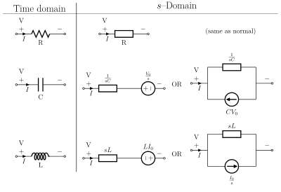
Note that the resistor is exactly the same in the time domain and the $s$ -domain. The sources are put in if there are initial conditions on the circuit elements. For example, if a capacitor has an initial voltage across it, or if the inductor has an initial current through it, the sources inserted in the $s$ -domain account for that.

The equivalents for current and voltage sources are simply derived from the transformations in the table above.

Examples: How to apply the properties and theorems

The Laplace transform is used frequently in engineering and physics; the output of a linear time-invariant system can be calculated by convolving its unit impulse response with the input signal. Performing this calculation in Laplace space turns the convolution into a multiplication; the latter being easier to solve because of its algebraic form. For more information, see control theory.

The Laplace transform can also be used to solve differential equations and is used extensively in electrical engineering. The Laplace transform reduces a linear differential equation to an algebraic equation, which can then be solved by the formal rules of algebra. The original differential equation can then be solved by applying the inverse Laplace transform. The English electrical engineer Oliver Heaviside first proposed a similar scheme, although without using the Laplace transform; and the resulting operational calculus is credited as the Heaviside calculus.

Example 1: Solving a differential equation

In nuclear physics, the following fundamental relationship governs radioactive decay: the number of radioactive atoms $N$ in a sample of a radioactive isotope decays at a rate proportional to $N$ . This leads to the first order linear differential equation

{\frac {dN}{dt}}=-\lambda N,

where $λ$ is the decay constant. The Laplace transform can be used to solve this equation.

Rearranging the equation to one side, we have

{\frac {dN}{dt}}+\lambda N=0.

Next, we take the Laplace transform of both sides of the equation:

\left(s{\tilde {N}}(s)-N_{0}\right)+\lambda {\tilde {N}}(s)=0,

where

{\tilde {N}}(s)={\mathcal {L}}\{N(t)\}

and

N_{0}=N(0).

Solving, we find

{\tilde {N}}(s)={\frac {N_{0}}{s+\lambda }}.

Finally, we take the inverse Laplace transform to find the general solution

{\begin{aligned}N(t)&={\mathcal {L}}^{-1}\{{\tilde {N}}(s)\}={\mathcal {L}}^{-1}\!\left\{{\frac {N_{0}}{s+\lambda }}\right\}\\&=\ N_{0}e^{-\lambda t},\end{aligned}}

which is indeed the correct form for radioactive decay.

Example 2: Deriving the complex impedance for a capacitor

In the theory of electrical circuits, the current flow in a capacitor is proportional to the capacitance and rate of change in the electrical potential (in SI units). Symbolically, this is expressed by the differential equation

i=C{dv \over dt},

where $C$ is the capacitance (in farads) of the capacitor, $i = i (t)$ is the electric current (in amperes) through the capacitor as a function of time, and $v = v (t)$ is the voltage (in volts) across the terminals of the capacitor, also as a function of time.

Taking the Laplace transform of this equation, we obtain

I(s)=C(sV(s)-V_{0}),

where

{\begin{aligned}I(s)&={\mathcal {L}}\{i(t)\},\\V(s)&={\mathcal {L}}\{v(t)\},\end{aligned}}

and

V_{0}=v(t)|_{t=0}.\,

Solving for $V (s)$ we have

V(s)={I(s) \over sC}+{V_{0} \over s}.

The definition of the complex impedance $Z$ (in ohms) is the ratio of the complex voltage $V$ divided by the complex current $I$ while holding the initial state $V 0$ at zero:

Z(s)=\left.{V(s) \over I(s)}\right|_{V_{0}=0}.

Using this definition and the previous equation, we find:

Z(s)={\frac {1}{sC}},

which is the correct expression for the complex impedance of a capacitor.

Example 3: Method of partial fraction expansion

Consider a linear time-invariant system with transfer function

H(s)={\frac {1}{(s+\alpha )(s+\beta )}}.

The impulse response is simply the inverse Laplace transform of this transfer function:

h(t)={\mathcal {L}}^{-1}\{H(s)\}.

To evaluate this inverse transform, we begin by expanding $H (s)$ using the method of partial fraction expansion,

{\frac {1}{(s+\alpha )(s+\beta )}}={P \over s+\alpha }+{R \over s+\beta }.

The unknown constants $P$ and $R$ are the residues located at the corresponding poles of the transfer function. Each residue represents the relative contribution of that singularity to the transfer function's overall shape.

By the residue theorem, the inverse Laplace transform depends only upon the poles and their residues. To find the residue $P$ , we multiply both sides of the equation by $s + α$ to get

{\frac {1}{s+\beta }}=P+{R(s+\alpha ) \over s+\beta }.

Then by letting $s = - α$ , the contribution from $R$ vanishes and all that is left is

P=\left.{1 \over s+\beta }\right|_{s=-\alpha }={1 \over \beta -\alpha }.

Similarly, the residue $R$ is given by

R=\left.{1 \over s+\alpha }\right|_{s=-\beta }={1 \over \alpha -\beta }.

Note that

R={-1 \over \beta -\alpha }=-P

and so the substitution of $R$ and $P$ into the expanded expression for $H (s)$ gives

H(s)=\left({\frac {1}{\beta -\alpha }}\right)\cdot \left({1 \over s+\alpha }-{1 \over s+\beta }\right).

Finally, using the linearity property and the known transform for exponential decay (see Item #3 in the Table of Laplace Transforms, above), we can take the inverse Laplace transform of $H (s)$ to obtain

h(t)={\mathcal {L}}^{-1}\{H(s)\}={\frac {1}{\beta -\alpha }}\left(e^{-\alpha t}-e^{-\beta t}\right),

which is the impulse response of the system.

Example 3.2: Convolution

The same result can be achieved using the convolution property as if the system is a series of filters with transfer functions of $1/(s + a)$ and $1/(s + b)$ . That is, the inverse of

H(s)={\frac {1}{(s+a)(s+b)}}={\frac {1}{s+a}}\cdot {\frac {1}{s+b}}

{\mathcal {L}}^{-1}\!\left\{{\frac {1}{s+a}}\right\}*{\mathcal {L}}^{-1}\!\left\{{\frac {1}{s+b}}\right\}=e^{-at}*e^{-bt}=\int _{0}^{t}e^{-ax}e^{-b(t-x)}\,dx={\frac {e^{-at}-e^{-bt}}{b-a}}.

Example 4: Mixing sines, cosines, and exponentials

Time function	Laplace transform
$e^{-\alpha t}\left[\cos {(\omega t)}+\left({\frac {\beta -\alpha }{\omega }}\right)\sin {(\omega t)}\right]u(t)$	${\frac {s+\beta }{(s+\alpha )^{2}+\omega ^{2}}}$

Starting with the Laplace transform

X(s)={\frac {s+\beta }{(s+\alpha )^{2}+\omega ^{2}}},

we find the inverse transform by first adding and subtracting the same constant $α$ to the numerator:

X(s)={\frac {s+\alpha }{(s+\alpha )^{2}+\omega ^{2}}}+{\frac {\beta -\alpha }{(s+\alpha )^{2}+\omega ^{2}}}.

By the shift-in-frequency property, we have

{\begin{aligned}x(t)&=e^{-\alpha t}{\mathcal {L}}^{-1}\left\{{s \over s^{2}+\omega ^{2}}+{\beta -\alpha \over s^{2}+\omega ^{2}}\right\}\\[8pt]&=e^{-\alpha t}{\mathcal {L}}^{-1}\left\{{s \over s^{2}+\omega ^{2}}+\left({\beta -\alpha \over \omega }\right)\left({\omega \over s^{2}+\omega ^{2}}\right)\right\}\\[8pt]&=e^{-\alpha t}\left[{\mathcal {L}}^{-1}\left\{{s \over s^{2}+\omega ^{2}}\right\}+\left({\beta -\alpha \over \omega }\right){\mathcal {L}}^{-1}\left\{{\omega \over s^{2}+\omega ^{2}}\right\}\right]\!.\end{aligned}}

Finally, using the Laplace transforms for sine and cosine (see the table, above), we have

{\begin{aligned}x(t)&=e^{-\alpha t}\left[\cos {(\omega t)}u(t)+\left({\frac {\beta -\alpha }{\omega }}\right)\sin {(\omega t)}u(t)\right].\\x(t)&=e^{-\alpha t}\left[\cos {(\omega t)}+\left({\frac {\beta -\alpha }{\omega }}\right)\sin {(\omega t)}\right]u(t).\end{aligned}}

Example 5: Phase delay

Time function	Laplace transform
$\sin {(\omega t+\phi )}$	${\frac {s\sin(\phi )+\omega \cos(\phi )}{s^{2}+\omega ^{2}}}$
$\cos {(\omega t+\phi )}$	${\frac {s\cos(\phi )-\omega \sin(\phi )}{s^{2}+\omega ^{2}}}.$

Starting with the Laplace transform,

X(s)={\frac {s\sin(\phi )+\omega \cos(\phi )}{s^{2}+\omega ^{2}}}

we find the inverse by first rearranging terms in the fraction:

{\begin{aligned}X(s)&={\frac {s\sin(\phi )}{s^{2}+\omega ^{2}}}+{\frac {\omega \cos(\phi )}{s^{2}+\omega ^{2}}}\\&=\sin(\phi )\left({\frac {s}{s^{2}+\omega ^{2}}}\right)+\cos(\phi )\left({\frac {\omega }{s^{2}+\omega ^{2}}}\right).\end{aligned}}

We are now able to take the inverse Laplace transform of our terms:

{\begin{aligned}x(t)&=\sin(\phi ){\mathcal {L}}^{-1}\left\{{\frac {s}{s^{2}+\omega ^{2}}}\right\}+\cos(\phi ){\mathcal {L}}^{-1}\left\{{\frac {\omega }{s^{2}+\omega ^{2}}}\right\}\\&=\sin(\phi )\cos(\omega t)+\sin(\omega t)\cos(\phi ).\end{aligned}}

This is just the sine of the sum of the arguments, yielding:

x(t)=\sin(\omega t+\phi ).

We can apply similar logic to find that

{\mathcal {L}}^{-1}\left\{{\frac {s\cos \phi -\omega \sin \phi }{s^{2}+\omega ^{2}}}\right\}=\cos {(\omega t+\phi )}.

Example 6: Determining structure of astronomical object from spectrum

The wide and general applicability of the Laplace transform and its inverse is illustrated by an application in astronomy which provides some information on the spatial distribution of matter of an astronomical source of radiofrequency thermal radiation too distant to resolve as more than a point, given its flux density spectrum, rather than relating the time domain with the spectrum (frequency domain).

Assuming certain properties of the object, e.g. spherical shape and constant temperature, calculations based on carrying out an inverse Laplace transformation on the spectrum of the object can produce the only possible model of the distribution of matter in it (density as a function of distance from the center) consistent with the spectrum.^[22] When independent information on the structure of an object is available, the inverse Laplace transform method has been found to be in good agreement.

Notes

↑ Korn & Korn 1967, §8.1
↑ Théorie des Probabilités 1812, 1825, chap.I sect.2-20 "On generating functions"
↑ An influential book was: M.F.Gardner & J.L.Barnes: Transients in Linear Systems studied by the Laplace Transform (1942) NY Wiley
↑ Euler 1744, Euler 1753, Euler 1769
↑ Lagrange 1773
↑ Grattan-Guinness 1997, p. 260
↑ Grattan-Guinness 1997, p. 261
↑ Grattan-Guinness 1997, pp. 261–262
↑ Grattan-Guinness 1997, pp. 262–266
↑ Feller 1971, §XIII.1
↑ The cumulative distribution function is the integral of the probability density function.
↑ Widder 1941, Chapter II, §1
↑ Widder 1941, Chapter VI, §2
↑ Korn & Korn 1967, pp. 226–227
↑ Bracewell 2000, Table 14.1, p. 385
↑ Feller 1971, p. 432
↑ Takacs 1953, p. 93
↑ Riley, K. F.; Hobson, M. P.; Bence, S. J. (2010), Mathematical methods for physics and engineering (3rd ed.), Cambridge University Press, p. 455, ISBN 978-0-521-86153-3
↑ Distefano, J. J.; Stubberud, A. R.; Williams, I. J. (1995), Feedback systems and control, Schaum's outlines (2nd ed.), McGraw-Hill, p. 78, ISBN 0-07-017052-5
↑ Lipschutz, S.; Spiegel, M. R.; Liu, J. (2009), Mathematical Handbook of Formulas and Tables, Schaum's Outline Series (3rd ed.), McGraw-Hill, p. 183, ISBN 978-0-07-154855-7 – provides the case for real $q$ .
↑ http://mathworld.wolfram.com/LaplaceTransform.html – Wolfram Mathword provides case for complex $q$
↑ Salem, M.; Seaton, M. J. (1974), "I. Continuum spectra and brightness contours", Monthly Notices of the Royal Astronomical Society, 167: 493–510, Bibcode:1974MNRAS.167..493S, doi:10.1093/mnras/167.3.493 , and
Salem, M. (1974), "II. Three-dimensional models", Monthly Notices of the Royal Astronomical Society, 167: 511–516, Bibcode:1974MNRAS.167..511S, doi:10.1093/mnras/167.3.511

References

Modern

Bracewell, Ronald N. (1978), The Fourier Transform and its Applications (2nd ed.), McGraw-Hill Kogakusha, ISBN 0-07-007013-X
Bracewell, R. N. (2000), The Fourier Transform and Its Applications (3rd ed.), Boston: McGraw-Hill, ISBN 0-07-116043-4
Feller, William (1971), An introduction to probability theory and its applications. Vol. II., Second edition, New York: John Wiley & Sons, MR 0270403
Korn, G. A.; Korn, T. M. (1967), Mathematical Handbook for Scientists and Engineers (2nd ed.), McGraw-Hill Companies, ISBN 0-07-035370-0
Widder, David Vernon (1941), The Laplace Transform, Princeton Mathematical Series, v. 6, Princeton University Press, MR 0005923
Williams, J. (1973), Laplace Transforms, Problem Solvers, George Allen & Unwin, ISBN 0-04-512021-8
Takacs, J. (1953), "Fourier amplitudok meghatarozasa operatorszamitassal", Magyar Hiradastechnika (in Hungarian), IV (7–8): 93–96

Historical

Euler, L. (1744), "De constructione aequationum" [The Construction of Equations], Opera omnia, 1st series (in Latin), 22: 150–161
Euler, L. (1753), "Methodus aequationes differentiales" [A Method for Solving Differential Equations], Opera omnia, 1st series (in Latin), 22: 181–213
Euler, L. (1992) [1769], "Institutiones calculi integralis, Volume 2" [Institutions of Integral Calculus], Opera omnia, 1st series (in Latin), Basel: Birkhäuser, 12, ISBN 978-3764314743 , Chapters 3–5
Euler, Leonhard (1769), Institutiones calculi integralis [Institutions of Integral Calculus] (in Latin), II, Paris: Petropoli, ch. 3–5, pp. 57–153
Grattan-Guinness, I (1997), "Laplace's integral solutions to partial differential equations", in Gillispie, C. C., Pierre Simon Laplace 1749–1827: A Life in Exact Science, Princeton: Princeton University Press, ISBN 0-691-01185-0
Lagrange, J. L. (1773), Mémoire sur l'utilité de la méthode, Œuvres de Lagrange, 2, pp. 171–234

External links

Wikimedia Commons has media related to Laplace transformation.

Hazewinkel, Michiel, ed. (2001), "Laplace transform", Encyclopedia of Mathematics, Springer, ISBN 978-1-55608-010-4
Online Computation of the transform or inverse transform, wims.unice.fr
Tables of Integral Transforms at EqWorld: The World of Mathematical Equations.
Weisstein, Eric W. "Laplace Transform". MathWorld.

Laplace Transform Module by John H. Mathews
Good explanations of the initial and final value theorems
Laplace Transforms at MathPages
Computational Knowledge Engine allows to easily calculate Laplace Transforms and its inverse Transform.

Authority control	NDL: 00567362

This article is issued from Wikipedia - version of the 11/15/2016. The text is available under the Creative Commons Attribution/Share Alike but additional terms may apply for the media files.

Laplace transform

History

Formal definition

Probability theory

Bilateral Laplace transform

Inverse Laplace transform

Region of convergence

Properties and theorems

Relation to power series

Relation to moments

Proof of the Laplace transform of a function's derivative

Evaluating integrals over the positive real axis

Evaluating improper integrals

Relationship to other transforms

Laplace–Stieltjes transform

Fourier transform

Mellin transform

Z-transform

Borel transform

Fundamental relationships

Table of selected Laplace transforms

s-domain equivalent circuits and impedances

Examples: How to apply the properties and theorems

Example 1: Solving a differential equation

Example 2: Deriving the complex impedance for a capacitor

Example 3: Method of partial fraction expansion

Example 3.2: Convolution

Example 4: Mixing sines, cosines, and exponentials

Example 5: Phase delay

Example 6: Determining structure of astronomical object from spectrum

See also

Notes

References

Modern

Historical

Further reading

External links