Interval arithmetic

Tolerance function (turquoise) and interval-valued approximation (red)

Interval arithmetic, interval mathematics, interval analysis, or interval computation, is a method developed by mathematicians since the 1950s and 1960s, as an approach to putting bounds on rounding errors and measurement errors in mathematical computation and thus developing numerical methods that yield reliable results. Very simply put, it represents each value as a range of possibilities. For example, instead of estimating the height of someone using standard arithmetic as 2.0 metres, using interval arithmetic we might be certain that that person is somewhere between 1.97 and 2.03 metres.

This concept is suitable for a variety of purposes. The most common use is to keep track of and handle rounding errors directly during the calculation and of uncertainties in the knowledge of the exact values of physical and technical parameters. The latter often arise from measurement errors and tolerances for components or due to limits on computational accuracy. Interval arithmetic also helps find reliable and guaranteed solutions to equations and optimization problems.

Mathematically, instead of working with an uncertain real $x$ we work with the two ends of the interval $[a,b]$ that contains $x$ . In interval arithmetic, any variable $x$ lies between $a$ and $b$ , or could be one of them. A function $f$ when applied to $x$ is also uncertain. In interval arithmetic $f$ produces an interval $[c,d]$ that is all the possible values for $f(x)$ for all $x\in [a,b]$ .

Introduction

The main focus of interval arithmetic is the simplest way to calculate upper and lower endpoints for the range of values of a function in one or more variables. These endpoints are not necessarily the supremum or infimum, since the precise calculation of those values can be difficult or impossible.

Treatment is typically limited to real intervals, so quantities of form

[a,b] = \{x \in \mathbb{R} \,|\, a \le x \le b\},

where $a = {-\infty}$ and $b = {\infty}$ are allowed; with one of them infinite we would have an unbounded interval, while with both infinite we would have the extended real number line.

As with traditional calculations with real numbers, simple arithmetic operations and functions on elementary intervals must first be defined.^[1] More complicated functions can be calculated from these basic elements.^[1]

Example

Body Mass Index for a person 1.80 m tall in relation to body weight m (in kilograms)

Take as an example the calculation of body mass index (BMI). The BMI is the body weight in kilograms divided by the square of height in metres. Measuring the mass with bathroom scales may have an accuracy of one kilogram. We do not know intermediate values – about 79.6 kg or 80.3 kg – but information rounded to the nearest whole number. It is unlikely that when the scale reads 80 kg, someone really weighs exactly 80.0 kg. In normal rounding to the nearest value, the scales showing 80 kg indicates a weight between 79.5 kg and 80.5 kg. The relevant range is that of all real numbers that are greater than or equal to 79.5, while less than or equal to 80.5, or in other words the interval [79.5,80.5].

For a man who weighs 80 kg and is 1.80 m tall, the BMI is about 24.7. With a weight of 79.5 kg and the same height the value is 24.5, while 80.5 kilograms gives almost 24.9. So the actual BMI is in the range [24.5,24.9]. The error in this case does not affect the conclusion (normal weight), but this is not always the position. For example, weight fluctuates in the course of a day so that the BMI can vary between 24 (normal weight) and 25 (overweight). Without detailed analysis it is not possible to always exclude questions as to whether an error ultimately is large enough to have significant influence.

Interval arithmetic states the range of possible outcomes explicitly. Simply put, results are no longer stated as numbers, but as intervals that represent imprecise values. The size of the intervals are similar to error bars to a metric in expressing the extent of uncertainty. Simple arithmetic operations, such as basic arithmetic and trigonometric functions, enable the calculation of outer limits of intervals.

Simple arithmetic

Body mass index for different weights in relation to height L (in metres)

Returning to the earlier BMI example, in determining the body mass index, height and body weight both affect the result. For height, measurements are usually in round centimetres: a recorded measurement of 1.80 metres actually means a height somewhere between 1.795 m and 1.805 m. This uncertainty must be combined with the fluctuation range in weight between 79.5 kg and 80.5 kg. The BMI is defined as the weight in kilograms divided by the square of height in metre. Using either 79.5 kg and 1.795 m or 80.5 kg and 1.805 m gives approximately 24.7. But the person in question may only be 1.795 m tall, with a weight of 80.5 kilograms – or 1.805 m and 79.5 kilograms: all combinations of all possible intermediate values must be considered. Using the interval arithmetic methods described below, the BMI lies in the interval

[79{.}5; 80{.}5]/([1{.}795; 1{.}805])^2 = [24{.}4; 25{.}0].

An operation ${\langle\!\mathrm{op}\!\rangle}$ , such as addition or multiplication, on two intervals is defined by

[x_1, x_2] {\,\langle\!\mathrm{op}\!\rangle\,} [y_1, y_2] = \{ x {\,\langle\!\mathrm{op}\!\rangle\,} y \, | \, x \in [x_1, x_2] \,\mbox{and}\, y \in [y_1, y_2] \}

For the four basic arithmetic operations this can become

\begin{align}[][x_1, x_2] \,\langle\!\mathrm{op}\!\rangle\, [y_1, y_2] & = \left[ \min(x_1 {\langle\!\mathrm{op}\!\rangle} y_1, x_1 \langle\!\mathrm{op}\!\rangle y_2, x_2 \langle\!\mathrm{op}\!\rangle y_1, x_2 \langle\!\mathrm{op}\!\rangle y_2), \right.\\ &{}\qquad \left. \;\max(x_1 {\langle\!\mathrm{op}\!\rangle}y_1, x_1 {\langle\!\mathrm{op}\!\rangle} y_2, x_2 {\langle\!\mathrm{op}\!\rangle} y_1, x_2 {\langle\!\mathrm{op}\!\rangle} y_2) \right] \,\mathrm{,} \end{align}

provided that $x {\,\langle\!\mathrm{op}\!\rangle\,} y$ is allowed for all $x\in [x_1, x_2]$ and $y \in [y_1, y_2]$ .

For practical applications this can be simplified further:

Addition: $[x_1, x_2] + [y_1, y_2] = [x_1+y_1, x_2+y_2]$
Subtraction: $[x_1, x_2] - [y_1, y_2] = [x_1-y_2, x_2-y_1]$
Multiplication: $[x_1, x_2] \cdot [y_1, y_2] = [\min(x_1 y_1,x_1 y_2,x_2 y_1,x_2 y_2), \max(x_1 y_1,x_1 y_2,x_2 y_1,x_2 y_2)]$
Division: $[x_1, x_2] / [y_1, y_2] = [x_1, x_2] \cdot (1/[y_1, y_2])$ , where $1/[y_1, y_2] = [1/y_2, 1/y_1]$ if $0 \notin [y_1, y_2]$ .

For division by an interval including zero, first define

1/[y_1, 0] = [-\infty, 1/y_1]

and

1/[0, y_2] = [1/y_2, \infty]

For $y_1 < 0 < y_2$ , we get $1/[y_1, y_2] = [-\infty, 1/y_1] \cup [1/y_2, \infty]$ , which as a single interval gives $1/[y_1, y_2] = [-\infty, \infty]$ . This loses useful information about $(1/y_1, 1/y_2)$ . So typically it is common to work with $[-\infty, 1/y_1]$ and $[1/y_2, \infty]$ as separate intervals.

Because several such divisions may occur in an interval arithmetic calculation, it is sometimes useful to do the calculation with so-called multi-intervals of the form $\textstyle \bigcup_{i=1}^l [x_{i1},x_{i2}]$ . The corresponding multi-interval arithmetic maintains a disjoint set of intervals and also provides for overlapping intervals to unite.^[2]

Since a real number $r\in \mathbb{R}$ can be interpreted as the interval $[r,r]$ , intervals and real numbers can be freely and easily combined.

With the help of these definitions, it is already possible to calculate the range of simple functions, such as $f(a,b,x) = a \cdot x + b$ . If, for example, $a = [1,2]$ , $b = [5,7]$ and $x = [2,3]$ , it is clear

f(a,b,x) = ([1,2] \cdot [2,3]) + [5,7] = [1\cdot 2, 2\cdot 3] + [5,7] = [7,13]

Interpreting this as a function $f(a,b,x)$ of the variable $x$ with interval parameters $a$ and $b$ , then it is possible to find the roots of this function. It is then

f([1,2],[5,7],x) = ([1,2] \cdot x) + [5,7] = 0\Leftrightarrow [1,2] \cdot x = [-7, -5]\Leftrightarrow x = [-7, -5]/[1,2],

the possible zeros are in the interval $[-7, {-2.5}]$ .

Multiplication of positive intervals

As in the above example, the multiplication of intervals often only requires two multiplications. It is in fact

[x_1, x_2] \cdot [y_1, y_2] = [x_1 \cdot y_1, x_2 \cdot y_2],\text{ if }x_1, y_1 \geq 0.

The multiplication can be seen as a destination area of a rectangle with varying edges. The result interval covers all levels from the smallest to the largest.

The same applies when one of the two intervals is non-positive and the other non-negative. Generally, multiplication can produce results as wide as $[-\infty, \infty]$ , for example if $0 \cdot \infty$ is squared. This also occurs, for example, in a division, if the numerator and denominator both contain zero.

Notation

To make the notation of intervals smaller in formulae, brackets can be used.

So we can use $[x] \equiv [x_1, x_2]$ to represent an interval. For the set of all finite intervals, we can use

[\mathbb{R}] := \big\{\, [x_1, x_2] \,|\, x_1 \leq x_2 \text{ and } x_1, x_2 \in \mathbb{R} \cup \{-\infty, \infty\} \big\}

as an abbreviation. For a vector of intervals $\big([x]_1, \ldots , [x]_n \big) \in [\mathbb{R}]^n$ we can also use a bold font: $[\mathbf{x}]$ .

Note that in such a compact notation, $[x]$ should not be confused between a so-called improper or single point interval $[x_1, x_1]$ and the lower and upper limit.

Elementary functions

Values of a monotonic function

Interval methods can also apply to functions that do not just use simple arithmetic, and we must also use other basic functions to redefine intervals, using already known monotonicity properties.

For monotonic functions in one variable, the range of values is also easy. If $f:\mathbb {R} \rightarrow \mathbb {R}$ is monotonically rising or falling in the interval $[x_1, x_2]$ , then for all values in the interval $y_1, y_2 \in [x_1, x_2]$ such that $y_1 \leq y_2$ , one of the following inequalities applies:

f(y_1) \leq f(y_2)

, or

f(y_1) \geq f(y_2)

The range corresponding to the interval $[y_1, y_2] \subseteq [x_1, x_2]$ can be calculated by applying the function to the endpoints $y_{1}$ and $y_{2}$ :

f([y_1, y_2]) = \left[\min \big \{f(y_1), f(y_2) \big\}, \max \big\{ f(y_1), f(y_2) \big\}\right]

From this the following basic features for interval functions can easily be defined:

Exponential function: $a^{[x_1, x_2]} = [a^{x_1},a^{x_2}]$ , for $a > 1$ ,
Logarithm: $\log_a\big( {[x_1, x_2]} \big) = [\log_a {x_1}, \log_a {x_2}]$ , for positive intervals $[x_1, x_2]$ and $a>1$
Odd powers: ${[x_1, x_2]}^n = [{x_1}^n,{x_2}^n]$ , for odd $n\in \mathbb{N}$ .

For even powers, the range of values being considered is important, and needs to be dealt with before doing any multiplication. For example, $x^{n}$ for $x \in [-1,1]$ should produce the interval $[0,1]$ when $n = 2, 4, 6, \ldots$ . But if $[-1,1]^n$ is taken by applying interval multiplication of form $[-1,1]\cdot \ldots \cdot [-1,1]$ then the result appears to be $[-1,1]$ , wider than necessary.

Instead consider the function $x^{n}$ as a monotonically decreasing function for $x<0$ and a monotonically increasing function for $x>0$ . So for even $n\in \mathbb{N}$ :

${[x_1, x_2]}^n = [x_1^n, x_2^n]$ , if $x_1 \geq 0$ ,
${[x_1, x_2]}^n = [x_2^n, x_1^n]$ , if $x_2 < 0$ ,
${[x_1, x_2]}^n = [0, \max \{x_1^n, x_2^n \} ]$ , otherwise.

More generally, one can say that for piecewise monotonic functions it is sufficient to consider the endpoints $x_{1},x_{2}$ of the interval $[x_1, x_2]$ , together with the so-called critical points within the interval being those points where the monotonicity of the function changes direction.

For the sine and cosine functions, the critical points are at $\left( {}^1\!\!/\!{}_2 + {n}\right) \cdot \pi$ or ${n} \cdot \pi$ for all $n \in \mathbb{Z}$ respectively. Only up to five points matter as the resulting interval is $[-1,1]$ if the interval includes at least two extrema. For sine and cosine, only the endpoints need full evaluation as the critical points lead to easily pre-calculated values – namely -1, 0, +1.

Interval extensions of general functions

In general, it may not be easy to find such a simple description of the output interval for many functions. But it may still be possible to extend functions to interval arithmetic. If $f:\mathbb{R}^n \rightarrow \mathbb{R}$ is a function from a real vector to a real number, then $[f]:[\mathbb{R}]^n \rightarrow [\mathbb{R}]$ is called an interval extension of $f$ if

[f]([\mathbf{x}]) \supseteq \{f(\mathbf{y}) | \mathbf{y} \in [\mathbf{x}]\}

This definition of the interval extension does not give a precise result. For example, both $[f]([x_1,x_2]) =[e^{x_1}, e^{x_2}]$ and $[g]([x_1,x_2]) =[{-\infty}, {\infty}]$ are allowable extensions of the exponential function. Extensions as tight as possible are desirable, taking into the relative costs of calculation and imprecision; in this case $[f]$ should be chosen as it give the tightest possible result.

The natural interval extension is achieved by combining the function rule $f(x_1, \cdots, x_n)$ with the equivalents of the basic arithmetic and elementary functions.

The Taylor interval extension (of degree $k$ ) is a $k+1$ times differentiable function $f$ defined by

[f]([\mathbf{x}]) := f(\mathbf{y}) + \sum_{i=1}^k\frac{1}{i!}\mathrm{D}^i f(\mathbf{y}) \cdot ([\mathbf{x}] - \mathbf{y})^i + [r]([\mathbf{x}], [\mathbf{x}], \mathbf{y})

for some $\mathbf{y} \in [\mathbf{x}]$ , where $\mathrm{D}^i f(\mathbf{y})$ is the $i$ th order differential of $f$ at the point $\mathbf {y}$ and $[r]$ is an interval extension of the Taylor remainder

r(\mathbf{x}, \xi, \mathbf{y}) = \frac{1}{(k+1)!}\mathrm{D}^{k+1} f(\xi) \cdot (\mathbf{x}-\mathbf{y})^{k+1}.

Mean value form

The vector $\xi$ lies between $\mathbf {x}$ and $\mathbf {y}$ with $\mathbf{x}, \mathbf{y} \in [\mathbf{x}]$ , $\xi$ is protected by $[\mathbf{x}]$ . Usually one chooses $\mathbf {y}$ to be the midpoint of the interval and uses the natural interval extension to assess the remainder.

The special case of the Taylor interval extension of degree $k=0$ is also referred to as the mean value form. For an interval extension of the Jacobian $[J_f](\mathbf{[x]})$ we get

[f]([\mathbf{x}]) := f(\mathbf{y}) + [J_f](\mathbf{[x]}) \cdot ([\mathbf{x}] - \mathbf{y})

A nonlinear function can be defined by linear features.

Complex interval arithmetic

An interval can also be defined as a locus of points at a given distance from the centre, and this definition can be extended from real numbers to complex numbers.^[3] As it is the case with computing with real numbers, computing with complex numbers involves uncertain data. So, given the fact that an interval number is a real closed interval and a complex number is an ordered pair of real numbers, there is no reason to limit the application of interval arithmetic to the measure of uncertainties in computations with real numbers.^[4] Interval arithmetic can thus be extended, via complex interval numbers, to determine regions of uncertainty in computing with complex numbers.^[4]

The basic algebraic operations for real interval numbers (real closed intervals) can be extended to complex numbers. It is therefore not surprising that complex interval arithmetic is similar to, but not the same as, ordinary complex arithmetic.^[4] It can be shown that, as it is the case with real interval arithmetic, there is no distributivity between addition and multiplication of complex interval numbers except for certain special cases, and inverse elements do not always exist for complex interval numbers.^[4] Two other useful properties of ordinary complex arithmetic fail to hold in complex interval arithmetic: the additive and multiplicative properties, of ordinary complex conjugates, do not hold for complex interval conjugates.^[4]

Interval arithmetic can be extended, in an analogous manner, to other multidimensional number systems such as quaternions and octonions, but with the expense that we have to sacrifice other useful properties of ordinary arithmetic.^[4]

Interval methods

The methods of classical numerical analysis can not be transferred one-to-one into interval-valued algorithms, as dependencies between numerical values are usually not taken into account.

Rounded interval arithmetic

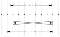
Outer bounds at different level of rounding

To work effectively in a real-life implementation, intervals must be compatible with floating point computing. The earlier operations were based on exact arithmetic, but in general fast numerical solution methods may not be available. The range of values of the function $f(x, y) = x + y$ for $x \in [0.1, 0.8]$ and $y \in [0.06, 0.08]$ are for example $[0.16, 0.88]$ . Where the same calculation is done with single digit precision, the result would normally be $[0.2, 0.9]$ . But $[0.2, 0.9] \not\supseteq [0.16, 0.88]$ , so this approach would contradict the basic principles of interval arithmetic, as a part of the domain of $f([0.1, 0.8], [0.06, 0.08])$ would be lost. Instead, the outward rounded solution $[0.1, 0.9]$ is used.

The standard IEEE 754 for binary floating-point arithmetic also sets out procedures for the implementation of rounding. An IEEE 754 compliant system allows programmers to round to the nearest floating point number; alternatives are rounding towards 0 (truncating), rounding toward positive infinity (i.e. up), or rounding towards negative infinity (i.e. down).

The required external rounding for interval arithmetic can thus be achieved by changing the rounding settings of the processor in the calculation of the upper limit (up) and lower limit (down). Alternatively, an appropriate small interval $[\varepsilon_1, \varepsilon_2]$ can be added.

Dependency problem

Approximate estimate of the value range

The so-called dependency problem is a major obstacle to the application of interval arithmetic. Although interval methods can determine the range of elementary arithmetic operations and functions very accurately, this is not always true with more complicated functions. If an interval occurs several times in a calculation using parameters, and each occurrence is taken independently then this can lead to an unwanted expansion of the resulting intervals.

Treating each occurrence of a variable independently

As an illustration, take the function $f$ defined by $f(x) = x^2 + x$ . The values of this function over the interval $[-1, 1]$ are really $[-1/4 , 2]$ . As the natural interval extension, it is calculated as $[-1, 1]^2 + [-1, 1] = [0,1] + [-1,1] = [-1,2]$ , which is slightly larger; we have instead calculated the infimum and supremum of the function $h(x, y)= x^2+y$ over $x,y \in [-1,1]$ . There is a better expression of $f$ in which the variable $x$ only appears once, namely by rewriting $f(x) = x^2 + x$ as addition and squaring in the quadratic $f(x) = \left(x + \frac{1}{2}\right)^2 -\frac{1}{4}$ .

So the suitable interval calculation is

\left([-1,1] + \frac{1}{2}\right)^2 -\frac{1}{4} = \left[-\frac{1}{2}, \frac{3}{2}\right]^2 -\frac{1}{4} = \left[0, \frac{9}{4}\right] -\frac{1}{4} = \left[-\frac{1}{4},2\right]

and gives the correct values.

In general, it can be shown that the exact range of values can be achieved, if each variable appears only once and if $f$ is continuous inside the box. However, not every function can be rewritten this way.

Wrapping effect

The dependency of the problem causing over-estimation of the value range can go as far as covering a large range, preventing more meaningful conclusions.

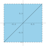
An additional increase in the range stems from the solution of areas that do not take the form of an interval vector. The solution set of the linear system

\begin{matrix} x &=& p\\ y &=& p \end{matrix}

for $p\in [-1,1]$ is precisely the line between the points $(-1,-1)$ and $(1,1)$ . Using interval methods results in the unit square, $[-1,1] \times [-1,1]$ . This is known as the wrapping effect.

Linear interval systems

A linear interval system consists of a matrix interval extension $[\mathbf{A}] \in [\mathbb{R}]^{n\times m}$ and an interval vector $[\mathbf{b}] \in [\mathbb{R}]^{n}$ . We want the smallest cuboid $[\mathbf{x}] \in [\mathbb{R}]^{m}$ , for all vectors $\mathbf{x} \in \mathbb{R}^{m}$ which there is a pair $(\mathbf{A}, \mathbf{b})$ with $\mathbf{A} \in [\mathbf{A}]$ and $\mathbf{b} \in [\mathbf{b}]$ satisfying

\mathbf{A} \cdot \mathbf{x} = \mathbf{b}

For quadratic systems – in other words, for $n = m$ – there can be such an interval vector $[\mathbf{x}]$ , which covers all possible solutions, found simply with the interval Gauss method. This replaces the numerical operations, in that the linear algebra method known as Gaussian elimination becomes its interval version. However, since this method uses the interval entities $[\mathbf{A}]$ and $[\mathbf{b}]$ repeatedly in the calculation, it can produce poor results for some problems. Hence using the result of the interval-valued Gauss only provides first rough estimates, since although it contains the entire solution set, it also has a large area outside it.

A rough solution $[\mathbf{x}]$ can often be improved by an interval version of the Gauss–Seidel method. The motivation for this is that the $i$ -th row of the interval extension of the linear equation

\begin{pmatrix} {[a_{11}]} & \cdots & {[a_{1n}]} \\ \vdots & \ddots & \vdots \\ {[a_{n1}]} & \cdots & {[a_{nn}]} \end{pmatrix} \cdot \begin{pmatrix} {x_1} \\ \vdots \\ {x_n} \end{pmatrix} = \begin{pmatrix} {[b_1]} \\ \vdots \\ {[b_n]} \end{pmatrix}

can be determined by the variable $x_{i}$ if the division $1/[a_{ii}]$ is allowed. It is therefore simultaneously

x_j \in [x_j]

and

x_j \in \frac{[b_i]- \sum\limits_{k \not= j} [a_{ik}] \cdot [x_k]}{[a_{ii}]}

So we can now replace $[x_j]$ by

[x_j] \cap \frac{[b_i]- \sum\limits_{k \not= j} [a_{ik}] \cdot [x_k]}{[a_{ii}]}

and so the vector $[\mathbf{x}]$ by each element. Since the procedure is more efficient for a diagonally dominant matrix, instead of the system $[\mathbf{A}]\cdot \mathbf{x} = [\mathbf{b}]\mbox{,}$ one can often try multiplying it by an appropriate rational matrix $\mathbf {M}$ with the resulting matrix equation

(\mathbf{M}\cdot[\mathbf{A}])\cdot \mathbf{x} = \mathbf{M}\cdot[\mathbf{b}]

left to solve. If one chooses, for example, $\mathbf{M} = \mathbf{A}^{-1}$ for the central matrix $\mathbf{A} \in [\mathbf{A}]$ , then $\mathbf{M} \cdot[\mathbf{A}]$ is outer extension of the identity matrix.

These methods only work well if the widths of the intervals occurring are sufficiently small. For wider intervals it can be useful to use an interval-linear system on finite (albeit large) real number equivalent linear systems. If all the matrices $\mathbf{A} \in [\mathbf{A}]$ are invertible, it is sufficient to consider all possible combinations (upper and lower) of the endpoints occurring in the intervals. The resulting problems can be resolved using conventional numerical methods. Interval arithmetic is still used to determine rounding errors.

This is only suitable for systems of smaller dimension, since with a fully occupied $n\times n$ matrix, $2^{n^2}$ real matrices need to be inverted, with $2^{n}$ vectors for the right hand side. This approach was developed by Jiri Rohn and is still being developed.^[5]

Interval Newton method

Reduction of the search area in the interval Newton step in "thick" functions

An interval variant of Newton's method for finding the zeros in an interval vector $[\mathbf{x}]$ can be derived from the average value extension.^[6] For an unknown vector $\mathbf{z}\in [\mathbf{x}]$ applied to $\mathbf{y}\in [\mathbf{x}]$ , gives

f(\mathbf{z}) \in f(\mathbf{y}) + [J_f](\mathbf{[x]}) \cdot (\mathbf{z} - \mathbf{y})

For a zero $\mathbf {z}$ , that is $f(z)=0$ , and thus must satisfy

f(\mathbf{y}) + [J_f](\mathbf{[x]}) \cdot (\mathbf{z} - \mathbf{y})=0

This is equivalent to $\mathbf{z} \in \mathbf{y} - [J_f](\mathbf{[x]})^{-1}\cdot f(\mathbf{y})$ . An outer estimate of $[J_f](\mathbf{[x]})^{-1}\cdot f(\mathbf{y}))$ can be determined using linear methods.

In each step of the interval Newton method, an approximate starting value $[\mathbf{x}]\in [\mathbb{R}]^n$ is replaced by $[\mathbf{x}]\cap \left(\mathbf{y} - [J_f](\mathbf{[x]})^{-1}\cdot f(\mathbf{y})\right)$ and so the result can be improved iteratively. In contrast to traditional methods, the interval method approaches the result by containing the zeros. This guarantees that the result produces all zeros in the initial range. Conversely, it proves that no zeros of $f$ were in the initial range $[\mathbf{x}]$ if a Newton step produces the empty set.

The method converges on all zeros in the starting region. Division by zero can lead to separation of distinct zeros, though the separation may not be complete; it can be complemented by the bisection method.

As an example, consider the function $f(x)= x^2-2$ , the starting range $[x] = [-2,2]$ , and the point $y= 0$ . We then have $J_f(x) = 2\, x$ and the first Newton step gives

[-2,2]\cap \left(0 - \frac{1}{2\cdot[-2,2]} (0-2)\right) = [-2,2]\cap \Big([{-\infty}, {-0.5}]\cup [{0.5}, {\infty}] \Big) = [{-2}, {-0.5}] \cup [{0.5}, {2}]

More Newton steps are used separately on $x\in [{-2}, {-0.5}]$ and $[{0.5}, {2}]$ . These converge to arbitrarily small intervals around $-{\sqrt {2}}$ and $+{\sqrt {2}}$ .

The Interval Newton method can also be used with thick functions such as $g(x)= x^2-[2,3]$ , which would in any case have interval results. The result then produces intervals containing $\left[-\sqrt{3},-\sqrt{2} \right] \cup \left[\sqrt{2},\sqrt{3} \right]$ .

Bisection and covers

Rough estimate (turquoise) and improved estimates through "mincing" (red)

The various interval methods deliver conservative results as dependencies between the sizes of different intervals extensions are not taken into account. However the dependency problem becomes less significant for narrower intervals.

Covering an interval vector $[\mathbf{x}]$ by smaller boxes $[\mathbf{x}_1], \dots , [\mathbf{x}_k]\mbox{,}$ so that $\textstyle [\mathbf{x}] = \bigcup_{i=1}^k [\mathbf{x}_i]\mbox{,}$ is then valid for the range of values $\textstyle f([\mathbf{x}]) = \bigcup_{i=1}^k f([\mathbf{x}_i])\mbox{.}$ So for the interval extensions described above, $\textstyle [f]([\mathbf{x}]) \supseteq \bigcup_{i=1}^k [f]([\mathbf{x}_i])$ is valid. Since $[f]([\mathbf{x}])$ is often a genuine superset of the right-hand side, this usually leads to an improved estimate.

Such a cover can be generated by the bisection method such as thick elements $[x_{i1}, x_{i2}]$ of the interval vector $[\mathbf{x}] = ([x_{11}, x_{12}], \dots, [x_{n1}, x_{n2}])$ by splitting in the centre into the two intervals $[x_{i1}, (x_{i1}+x_{i2})/2]$ and $[(x_{i1}+x_{i2})/2, x_{i2}]$ . If the result is still not suitable then further gradual subdivision is possible. Note that a cover of $2^r$ intervals results from $r$ divisions of vector elements, substantially increasing the computation costs.

With very wide intervals, it can be helpful to split all intervals into several subintervals with a constant (and smaller) width, a method known as mincing. This then avoids the calculations for intermediate bisection steps. Both methods are only suitable for problems of low dimension.

Application

Interval arithmetic can be used in various areas (such as set inversion, motion planning, set estimation or stability analysis) to treat estimates with no exact numerical value.^[7]

Rounding error analysis

Interval arithmetic is used with error analysis, to control rounding errors arising from each calculation. The advantage of interval arithmetic is that after each operation there is an interval that reliably includes the true result. The distance between the interval boundaries gives the current calculation of rounding errors directly:

Error =

\mathrm{abs}(a-b)

for a given interval

[a,b]

Interval analysis adds to rather than substituting for traditional methods for error reduction, such as pivoting.

Tolerance analysis

Parameters for which no exact figures can be allocated often arise during the simulation of technical and physical processes. The production process of technical components allows certain tolerances, so some parameters fluctuate within intervals. In addition, many fundamental constants are not known precisely.^[2]

If the behavior of such a system affected by tolerances satisfies, for example, $f(\mathbf{x}, \mathbf{p}) = 0$ , for $\mathbf{p} \in [\mathbf{p}]$ and unknown $\mathbf {x}$ then the set of possible solutions

\{\mathbf{x}\,|\, \exists \mathbf{p} \in [\mathbf{p}], f(\mathbf{x}, \mathbf{p})= 0\}

can be found by interval methods. This provides an alternative to traditional propagation of error analysis. Unlike point methods, such as Monte Carlo simulation, interval arithmetic methodology ensures that no part of the solution area can be overlooked. However, the result is always a worst case analysis for the distribution of error, as other probability-based distributions are not considered.

Fuzzy interval arithmetic

Approximation of the normal distribution by a sequence of intervals

Interval arithmetic can also be used with affiliation functions for fuzzy quantities as they are used in fuzzy logic. Apart from the strict statements $x\in [x]$ and $x \not\in [x]$ , intermediate values are also possible, to which real numbers $\mu \in [0,1]$ are assigned. $\mu = 1$ corresponds to definite membership while $\mu =0$ is non-membership. A distribution function assigns uncertainty, which can be understood as a further interval.

For fuzzy arithmetic^[8] only a finite number of discrete affiliation stages $\mu_i \in [0,1]$ are considered. The form of such a distribution for an indistinct value can then represented by a sequence of intervals

\left[x^{(1)}\right] \supset \left[x^{(2)}\right] \supset \cdots \supset \left[x^{(k)} \right]

. The interval

[x^{(i)}]

corresponds exactly to the fluctuation range for the stage

\mu _{i}

The appropriate distribution for a function $f(x_1, \cdots, x_n)$ concerning indistinct values $x_1, \cdots, x_n$ and the corresponding sequences $\left[x_1^{(1)} \right] \supset \cdots \supset \left[x_1^{(k)} \right], \cdots , \left[x_n^{(1)} \right] \supset \cdots \supset \left[x_n^{(k)} \right]$ can be approximated by the sequence $\left[y^{(1)}\right] \supset \cdots \supset \left[y^{(k)}\right]$ . The values $\left[y^{(i)}\right]$ are given by $\left[y^{(i)}\right] = f \left( \left[x_{1}^{(i)}\right], \cdots \left[x_{n}^{(i)}\right]\right)$ and can be calculated by interval methods. The value $\left[y^{(1)}\right]$ corresponds to the result of an interval calculation.

History

Interval arithmetic is not a completely new phenomenon in mathematics; it has appeared several times under different names in the course of history. For example, Archimedes calculated lower and upper bounds 223/71 < π < 22/7 in the 3rd century BC. Actual calculation with intervals has neither been as popular as other numerical techniques, nor been completely forgotten.

Rules for calculating with intervals and other subsets of the real numbers were published in a 1931 work by Rosalind Cicely Young, a doctoral candidate at the University of Cambridge. Arithmetic work on range numbers to improve reliability of digital systems were then published in a 1951 textbook on linear algebra by Paul Dwyer (University of Michigan); intervals were used to measure rounding errors associated with floating-point numbers. A comprehensive paper on interval algebra in numerical analysis was published by Teruo Sunaga (1958).^[9]

The birth of modern interval arithmetic was marked by the appearance of the book Interval Analysis by Ramon E. Moore in 1966.^[10]^[11] He had the idea in Spring 1958, and a year later he published an article about computer interval arithmetic.^[12] Its merit was that starting with a simple principle, it provided a general method for automated error analysis, not just errors resulting from rounding.

Independently in 1956, Mieczyslaw Warmus suggested formulae for calculations with intervals,^[13] though Moore found the first non-trivial applications.

In the following twenty years, German groups of researchers carried out pioneering work around Götz Alefeld^[14] and Ulrich Kulisch^[1]^[15] at the University of Karlsruhe and later also at the Bergische University of Wuppertal. For example, Karl Nickel explored more effective implementations, while improved containment procedures for the solution set of systems of equations were due to Arnold Neumaier among others. In the 1960s, Eldon R. Hansen dealt with interval extensions for linear equations and then provided crucial contributions to global optimisation, including what is now known as Hansen's method, perhaps the most widely used interval algorithm.^[6] Classical methods in this often have the problem of determining the largest (or smallest) global value, but could only find a local optimum and could not find better values; Helmut Ratschek and Jon George Rokne developed branch and bound methods, which until then had only applied to integer values, by using intervals to provide applications for continuous values.

In 1988, Rudolf Lohner developed Fortran-based software for reliable solutions for initial value problems using ordinary differential equations.^[16]

The journal Reliable Computing (originally Interval Computations) has been published since the 1990s, dedicated to the reliability of computer-aided computations. As lead editor, R. Baker Kearfott, in addition to his work on global optimisation, has contributed significantly to the unification of notation and terminology used in interval arithmetic (Web: Kearfott).

In recent years work has concentrated in particular on the estimation of preimages of parameterised functions and to robust control theory by the COPRIN working group of INRIA in Sophia Antipolis in France (Web: INRIA).

Implementations

There are many software packages that permit the development of numerical applications using interval arithmetic.^[17] These are usually provided in the form of program libraries. There are also C++ and Fortran compilers that handle interval data types and suitable operations as a language extension, so interval arithmetic is supported directly.

Since 1967, Extensions for Scientific Computation (XSC) have been developed in the University of Karlsruhe for various programming languages, such as C++, Fortran and Pascal.^[18] The first platform was a Zuse Z 23, for which a new interval data type with appropriate elementary operators was made available. There followed in 1976, Pascal-SC, a Pascal variant on a Zilog Z80 that it made possible to create fast, complicated routines for automated result verification. Then came the Fortran 77-based ACRITH-XSC for the System/370 architecture (FORTRAN-SC), which was later delivered by IBM. Starting from 1991 one could produce code for C compilers with Pascal-XSC; a year later the C++ class library supported C-XSC on many different computer systems. In 1997, all XSC variants were made available under the GNU General Public License. At the beginning of 2000 C-XSC 2.0 was released under the leadership of the working group for scientific computation at the Bergische University of Wuppertal to correspond to the improved C++ standard.

Another C++-class library was created in 1993 at the Hamburg University of Technology called Profil/BIAS (Programmer's Runtime Optimized Fast Interval Library, Basic Interval Arithmetic), which made the usual interval operations more user friendly. It emphasized the efficient use of hardware, portability and independence of a particular presentation of intervals.

The Boost collection of C++ libraries contains a template class for intervals. Its authors are aiming to have interval arithmetic in the standard C++ language.^[19]

Gaol^[20] is another C++ interval arithmetic library that is unique in that it offers the relational interval operators used in interval constraint programming.

The Frink programming language has an implementation of interval arithmetic that handles arbitrary-precision numbers. Programs written in Frink can use intervals without rewriting or recompilation.

In addition computer algebra systems, such as Mathematica, Maple and MuPAD, can handle intervals. A Matlab extension Intlab builds on BLAS routines, and the Toolbox b4m makes a Profil/BIAS interface.^[21] Moreover, the Software Euler Math Toolbox includes an interval arithmetic.

A library for the functional language OCaml was written in assembly language and C.^[22]

IEEE Std 1788-2015 – IEEE standard for interval arithmetic

A standard for interval arithmetic has been approved in June 2015.^[23] Two reference implementations are freely available.^[24] These have been developed by members of the standard's working group: The libieeep1788^[25] library for C++, and the interval package^[26] for GNU Octave.

A minimal subset of the standard is currently under development that should be easier to implement and may speed production of implementations.^[27]

Conferences and Workshop

Several international conferences or workshop take place every year in the world. The main conference is probably SCAN (International Symposium on Scientific Computing, Computer Arithmetic, and Verified Numerical Computation), but there is also SWIM (Small Workshop on Interval Methods), PPAM (International Conference on Parallel Processing and Applied Mathematics), REC (International Workshop on Reliable Engineering Computing).

References

1 2 3 Kulisch, Ulrich (1989). Wissenschaftliches Rechnen mit Ergebnisverifikation. Eine Einführung (in German). Wiesbaden: Vieweg-Verlag. ISBN 3-528-08943-1.
1 2 Dreyer, Alexander (2003). Interval Analysis of Analog Circuits with Component Tolerances. Aachen, Germany: Shaker Verlag. ISBN 3-8322-4555-3.
↑ Complex interval arithmetic and its applications, Miodrag Petkovi?, Ljiljana Petkovi?, Wiley-VCH, 1998, ISBN 978-3-527-40134-5
1 2 3 4 5 6 Hend Dawood (2011). Theories of Interval Arithmetic: Mathematical Foundations and Applications. Saarbrücken: LAP LAMBERT Academic Publishing. ISBN 978-3-8465-0154-2.
↑ Jiri Rohn, List of publications
1 2 Walster, G. William; Hansen, Eldon Robert (2004). Global Optimization using Interval Analysis (2nd ed.). New York, USA: Marcel Dekker. ISBN 0-8247-4059-9.
↑ Jaulin, Luc; Kieffer, Michel; Didrit, Olivier; Walter, Eric (2001). Applied Interval Analysis. Berlin: Springer. ISBN 1-85233-219-0.
↑ Application of Fuzzy Arithmetic to Quantifying the Effects of Uncertain Model Parameters, Michael Hanss, University of Stuttgart
↑ Sunaga, Teruo (1958). Theory of interval algebra and its application to numerical analysis. RAAG Memoirs. pp. 29–46.
↑ Moore, R. E. (1966). Interval Analysis. Englewood Cliff, New Jersey, USA: Prentice-Hall. ISBN 0-13-476853-1.
↑ Cloud, Michael J.; Moore, Ramon E.; Kearfott, R. Baker (2009). Introduction to Interval Analysis. Philadelphia: Society for Industrial and Applied Mathematics (SIAM). ISBN 0-89871-669-1.
↑ Hansen, E. R. (2001-08-13). "Publications Related to Early Interval Work of R. E. Moore". University of Louisiana at Lafayette Press. Retrieved 2015-06-29.
↑ Precursory papers on interval analysis by M. Warmus Archived April 18, 2008, at the Wayback Machine.
↑ Alefeld, Götz; Herzberger, Jürgen. Einführung in die Intervallrechnung. Reihe Informatik (in German). 12. Mannheim, Wien, Zürich: B.I.-Wissenschaftsverlag. ISBN 3-411-01466-0.
↑ Kulisch, Ulrich (1969). "Grundzüge der Intervallrechnung". In Laugwitz, Detlef. Jahrbuch Überblicke Mathematik (in German). 2. Mannheim, Germany: Bibliographisches Institut. pp. 51–98.
↑ Bounds for ordinary differential equations of Rudolf Lohner (in German)
↑ Software for Interval Computations collected by Vladik Kreinovich , University of Texas at El Paso
↑ History of XSC-Languages
↑ A Proposal to add Interval Arithmetic to the C++ Standard Library
↑ Gaol is Not Just Another Interval Arithmetic Library
↑ INTerval LABoratory and b4m
↑ Alliot, Jean-Marc; Gotteland, Jean-Baptiste; Vanaret, Charlie; Durand, Nicolas; Gianazza, David (2012), Implementing an interval computation library for OCaml on x86/amd64 architectures, 17th ACM SIGPLAN International Conference on Functional Programming
↑ IEEE Standard for Interval Arithmetic
↑ Revol, Nathalie (2015). The (near-)future IEEE 1788 standard for interval arithmetic. 8th small workshop on interval methods. Slides (PDF)
↑ C++ implementation of the preliminary IEEE P1788 standard for interval arithmetic
↑ GNU Octave interval package
↑ "P1788.1 - Standard for Interval Arithmetic (Simplified)". IEEE Project. IEEE Standards Association. Retrieved 2016-08-16.
↑ Ball arithmetic by Joris van der Hoeven

External links

Data types

Uninterpreted	Bit Byte Trit Tryte Word Bit array

Numeric	Arbitrary-precision or bignum Complex Decimal Fixed point Floating point Double precision Extended precision Half precision Long double Minifloat Octuple precision Quadruple precision Single precision Integer signedness Interval Rational

Text	Character String null-terminated

Pointer	Address physical virtual Reference

Composite	Algebraic data type generalized Array Associative array Class Dependent Equality Inductive List Object metaobject Option type Product Record Set Union tagged

Other	Boolean Bottom type Collection Enumerated type Exception Function type Opaque data type Recursive data type Semaphore Stream Top type Type class Unit type Void

Related topics	Abstract data type Data structure Generic Kind metaclass Parametric polymorphism Primitive data type Protocol interface Subtyping Type constructor Type conversion Type system

See also platform-dependent and independent units of information

This article is issued from Wikipedia - version of the 11/30/2016. The text is available under the Creative Commons Attribution/Share Alike but additional terms may apply for the media files.