Insertion sort
 Graphical illustration of insertion sort | |
| Class | Sorting algorithm |
|---|---|
| Data structure | Array |
| Worst-case performance | О(n2) comparisons, swaps |
| Best-case performance | O(n) comparisons, O(1) swaps |
| Average performance | О(n2) comparisons, swaps |
| Worst-case space complexity | О(n) total, O(1) auxiliary |
Insertion sort is a simple sorting algorithm that builds the final sorted array (or list) one item at a time. It is much less efficient on large lists than more advanced algorithms such as quicksort, heapsort, or merge sort. However, insertion sort provides several advantages:
- Simple implementation: Bentley shows a three-line C version, and a five-line optimized version[1]:116
- Efficient for (quite) small data sets, much like other quadratic sorting algorithms
- More efficient in practice than most other simple quadratic (i.e., O(n2)) algorithms such as selection sort or bubble sort
- Adaptive, i.e., efficient for data sets that are already substantially sorted: the time complexity is O(nk) when each element in the input is no more than k places away from its sorted position
- Stable; i.e., does not change the relative order of elements with equal keys
- In-place; i.e., only requires a constant amount O(1) of additional memory space
- Online; i.e., can sort a list as it receives it
When people manually sort cards in a bridge hand, most use a method that is similar to insertion sort.[2]
Algorithm for insertion sort

Insertion sort iterates, consuming one input element each repetition, and growing a sorted output list. Each iteration, insertion sort removes one element from the input data, finds the location it belongs within the sorted list, and inserts it there. It repeats until no input elements remain.
Sorting is typically done in-place, by iterating up the array, growing the sorted list behind it. At each array-position, it checks the value there against the largest value in the sorted list (which happens to be next to it, in the previous array-position checked). If larger, it leaves the element in place and moves to the next. If smaller, it finds the correct position within the sorted list, shifts all the larger values up to make a space, and inserts into that correct position.
The resulting array after k iterations has the property where the first k + 1 entries are sorted ("+1" because the first entry is skipped). In each iteration the first remaining entry of the input is removed, and inserted into the result at the correct position, thus extending the result:
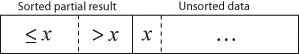
becomes

with each element greater than x copied to the right as it is compared against x.
The most common variant of insertion sort, which operates on arrays, can be described as follows:
- Suppose there exists a function called Insert designed to insert a value into a sorted sequence at the beginning of an array. It operates by beginning at the end of the sequence and shifting each element one place to the right until a suitable position is found for the new element. The function has the side effect of overwriting the value stored immediately after the sorted sequence in the array.
- To perform an insertion sort, begin at the left-most element of the array and invoke Insert to insert each element encountered into its correct position. The ordered sequence into which the element is inserted is stored at the beginning of the array in the set of indices already examined. Each insertion overwrites a single value: the value being inserted.
Pseudocode of the complete algorithm follows, where the arrays are zero-based:[1]:116
for i ← 1 to length(A)
    j ← i
    while j > 0 and A[j-1] > A[j]
        swap A[j] and A[j-1]
        j ← j - 1
    end while
end for
The outer loop runs over all the elements except the first one, because the single-element prefix A[0:1] is trivially sorted, so the invariant that the first i+1 entries are sorted is true from the start. The inner loop moves element A[i] to its correct place so that after the loop, the first i+2 elements are sorted.
After expanding the "swap" operation in-place as t ← A[j]; A[j] ← A[j-1]; A[j-1] ← t (where t is a temporary variable), a slightly faster version can be produced that moves A[i] to its position in one go and only performs one assignment in the inner loop body:[1]:116
 for i = 1 to length(A)
    x = A[i]
    j = i - 1
    while j >= 0 and A[j] > x
        A[j+1] = A[j]
        j = j - 1
    end while
    A[j+1] = x[3]
 end for
The new inner loop shifts elements to the right to clear a spot for x = A[i].
Note that although the common practice is to implement in-place, which requires checking the elements in-order, the order of checking (and removing) input elements is actually arbitrary. The choice can be made using almost any pattern, as long as all input elements are eventually checked (and removed from the input).
Best, worst, and average cases

The best case input is an array that is already sorted. In this case insertion sort has a linear running time (i.e., O(n)). During each iteration, the first remaining element of the input is only compared with the right-most element of the sorted subsection of the array.
The simplest worst case input is an array sorted in reverse order. The set of all worst case inputs consists of all arrays where each element is the smallest or second-smallest of the elements before it. In these cases every iteration of the inner loop will scan and shift the entire sorted subsection of the array before inserting the next element. This gives insertion sort a quadratic running time (i.e., O(n2)).
The average case is also quadratic, which makes insertion sort impractical for sorting large arrays. However, insertion sort is one of the fastest algorithms for sorting very small arrays, even faster than quicksort; indeed, good quicksort implementations use insertion sort for arrays smaller than a certain threshold, also when arising as subproblems; the exact threshold must be determined experimentally and depends on the machine, but is commonly around ten.
Example: The following table shows the steps for sorting the sequence {3, 7, 4, 9, 5, 2, 6, 1}. In each step, the key under consideration is underlined. The key that was moved (or left in place because it was biggest yet considered) in the previous step is shown in bold.
3 7 4 9 5 2 6 1
3 7 4 9 5 2 6 1
3 7 4 9 5 2 6 1
3 4 7 9 5 2 6 1
3 4 7 9 5 2 6 1
3 4 5 7 9 2 6 1
2 3 4 5 7 9 6 1
2 3 4 5 6 7 9 1
1 2 3 4 5 6 7 9
Relation to other sorting algorithms
Insertion sort is very similar to selection sort. As in selection sort, after k passes through the array, the first k elements are in sorted order. For selection sort these are the k smallest elements, while in insertion sort they are whatever the first k elements were in the unsorted array. Insertion sort's advantage is that it only scans as many elements as needed to determine the correct location of the k+1st element, while selection sort must scan all remaining elements to find the absolute smallest element.
Assuming the k+1st element's rank is random, insertion sort will on average require shifting half of the previous k elements, while selection sort always requires scanning all unplaced elements. So for unsorted input, insertion sort will usually perform about half as many comparisons as selection sort. If the input array is reverse-sorted, insertion sort performs as many comparisons as selection sort. If the input array is already sorted, insertion sort performs as few as n-1 comparisons, thus making insertion sort more efficient when given sorted or "nearly sorted" arrays.
While insertion sort typically makes fewer comparisons than selection sort, it requires more writes because the inner loop can require shifting large sections of the sorted portion of the array. In general, insertion sort will write to the array O(n2) times, whereas selection sort will write only O(n) times. For this reason selection sort may be preferable in cases where writing to memory is significantly more expensive than reading, such as with EEPROM or flash memory.
Some divide-and-conquer algorithms such as quicksort and mergesort sort by recursively dividing the list into smaller sublists which are then sorted. A useful optimization in practice for these algorithms is to use insertion sort for sorting small sublists, where insertion sort outperforms these more complex algorithms. The size of list for which insertion sort has the advantage varies by environment and implementation, but is typically between eight and twenty elements. A variant of this scheme runs quicksort with a constant cutoff K, then runs a single insertion sort on the final array:
proc quicksort_k(A, lo, hi)
    if hi - lo < K
        return
    pivot ← partition(A, lo, hi)
    quicksort_k(A, lo, pivot-1)
    quicksort_k(A, pivot + 1, hi)
proc sort(A)
    quicksort_k(A, 0, length(A))
    insertionsort(A)
This preserves the O(n lg n) expected time complexity of standard quicksort, because after running the quicksort_k procedure, the array A will be partially sorted in the sense that each element is at most K positions away from its final, sorted position. On such a partially sorted array, insertion sort will run at most K iterations of its inner loop, which is run n-1 times, so it has linear time complexity.[1]:121
Variants
D.L. Shell made substantial improvements to the algorithm; the modified version is called Shell sort. The sorting algorithm compares elements separated by a distance that decreases on each pass. Shell sort has distinctly improved running times in practical work, with two simple variants requiring O(n3/2) and O(n4/3) running time.
If the cost of comparisons exceeds the cost of swaps, as is the case for example with string keys stored by reference or with human interaction (such as choosing one of a pair displayed side-by-side), then using binary insertion sort may yield better performance. Binary insertion sort employs a binary search to determine the correct location to insert new elements, and therefore performs ⌈log2(n)⌉ comparisons in the worst case, which is O(n log n). The algorithm as a whole still has a running time of O(n2) on average because of the series of swaps required for each insertion.
The number of swaps can be reduced by calculating the position of multiple elements before moving them. For example, if the target position of two elements is calculated before they are moved into the right position, the number of swaps can be reduced by about 25% for random data. In the extreme case, this variant works similar to merge sort.
A variant named binary merge sort uses a binary insertion sort to sort groups of 32 elements, followed by a final sort using merge sort. It combines the speed of insertion sort on small data sets with the speed of merge sort on large data sets.[4]
To avoid having to make a series of swaps for each insertion, the input could be stored in a linked list, which allows elements to be spliced into or out of the list in constant-time when the position in the list is known. However, searching a linked list requires sequentially following the links to the desired position: a linked list does not have random access, so it cannot use a faster method such as binary search. Therefore, the running time required for searching is O(n) and the time for sorting is O(n2). If a more sophisticated data structure (e.g., heap or binary tree) is used, the time required for searching and insertion can be reduced significantly; this is the essence of heap sort and binary tree sort.
In 2006 Bender, Martin Farach-Colton, and Mosteiro published a new variant of insertion sort called library sort or gapped insertion sort that leaves a small number of unused spaces (i.e., "gaps") spread throughout the array. The benefit is that insertions need only shift elements over until a gap is reached. The authors show that this sorting algorithm runs with high probability in O(n log n) time.[5]
If a skip list is used, the insertion time is brought down to O(log n), and swaps are not needed because the skip list is implemented on a linked list structure. The final running time for insertion would be O(n log n).
List insertion sort is a variant of insertion sort. It reduces the number of movements.
List insertion sort code in C
If the items are stored in a linked list, then the list can be sorted with O(1) additional space. The algorithm starts with an initially empty (and therefore trivially sorted) list. The input items are taken off the list one at a time, and then inserted in the proper place in the sorted list. When the input list is empty, the sorted list has the desired result.
struct LIST * SortList1(struct LIST * pList)
{
    // zero or one element in list
    if(pList == NULL || pList->pNext == NULL)
        return pList;
    // head is the first element of resulting sorted list
    struct LIST * head = NULL;
    while(pList != NULL) {
        struct LIST * current = pList;
        pList = pList->pNext;
        if(head == NULL || current->iValue < head->iValue) {
            // insert into the head of the sorted list
            // or as the first element into an empty sorted list
            current->pNext = head;
            head = current;
        } else {
            // insert current element into proper position in non-empty sorted list
            struct LIST * p = head;
            while(p != NULL) {
                if(p->pNext == NULL || // last element of the sorted list
                   current->iValue < p->pNext->iValue) // middle of the list
                {
                    // insert into middle of the sorted list or as the last element
                    current->pNext = p->pNext;
                    p->pNext = current;
                    break; // done
                }
                p = p->pNext;
            }
        }
    }
    return head;
}
The algorithm below uses a trailing pointer[6] for the insertion into the sorted list. A simpler recursive method rebuilds the list each time (rather than splicing) and can use O(n) stack space.
struct LIST
{
  struct LIST * pNext;
  int           iValue;
};

struct LIST * SortList(struct LIST * pList)
{
  // zero or one element in list
  if(!pList || !pList->pNext)
      return pList;

  /* build up the sorted array from the empty list */
  struct LIST * pSorted = NULL;

  /* take items off the input list one by one until empty */
  while (pList != NULL)
  {
      /* remember the head */
      struct LIST *   pHead  = pList;
      /* trailing pointer for efficient splice */
      struct LIST ** ppTrail = &pSorted;

      /* pop head off list */
      pList = pList->pNext;

      /* splice head into sorted list at proper place */
      while (!(*ppTrail == NULL || pHead->iValue < (*ppTrail)->iValue)) /* does head belong here? */
      {
          /* no - continue down the list */
          ppTrail = &(*ppTrail)->pNext;
      }

      pHead->pNext = *ppTrail;
      *ppTrail = pHead;
  }

  return pSorted;
}
References
- 1 2 3 4 Bentley, Jon (2000). Programming Pearls. ACM Press/Addison–Wesley.
- ↑ Sedgewick, Robert (1983), Algorithms, Addison-Wesley, pp. 95ff, ISBN 978-0-201-06672-2.
- ↑ Cormen, Thomas H.; Leiserson, Charles E.; Rivest, Ronald L.; Stein, Clifford (2001) [1990]. Introduction to Algorithms (2nd ed.). MIT Press and McGraw-Hill. ISBN 0-262-03293-7. Section 2.1: Insertion sort, pp. 15–21. See in particular p. 17.
- ↑ "Binary Merge Sort".
- ↑ Bender, Michael A.; Farach-Colton, Martín; Mosteiro, Miguel A. (2006), "Insertion sort is O(n log n)", Theory of Computing Systems, 39 (3): 391–397, doi:10.1007/s00224-005-1237-z, MR 2218409
- ↑ Hill, Curt (ed.), "Trailing Pointer Technique", Euler, Valley City State University, retrieved 22 September 2012.
Additional reading
- Knuth, Donald (1998), "5.2.1: Sorting by Insertion", The Art of Computer Programming, 3. Sorting and Searching (second ed.), Addison-Wesley, pp. 80–105, ISBN 0-201-89685-0.
External links
| The Wikibook Algorithm implementation has a page on the topic of: Insertion sort |
| Wikimedia Commons has media related to Insertion sort. |
- Adamovsky, John Paul, Binary Insertion Sort – Scoreboard – Complete Investigation and C Implementation, Pathcom.
- Insertion Sort in C with demo, Electrofriends.
- Insertion Sort – a comparison with other O(n^2) sorting algorithms, UK: Core war.
- Category:Insertion Sort (wiki), LiteratePrograms – implementations of insertion sort in various programming languages
- InsertionSort, Code raptors – colored, graphical Java applet that allows experimentation with the initial input and provides statistics
- Harrison, Sorting Algorithms Demo, CA: UBC – visual demonstrations of sorting algorithms (implemented in Java)
- Insertion sort (illustrated explanation), Algo list. Java and C++ implementations.