IS–LM model
The IS–LM model, or Hicks–Hansen model, is a macroeconomic tool that shows the relationship between interest rates (ordinate) and assets market (also known as real output in goods and services market plus money market, as abscissa). The intersection of the "investment–saving" (IS) and "liquidity preference–money supply" (LM) curves models "general equilibrium" where supposed simultaneous equilibrium occurs in both interest and assets markets.[1] Yet two equivalent interpretations are possible: first, the IS–LM model explains changes in national income when price level is fixed short-run; second, the IS–LM model shows why an aggregate demand curve can shift.[2] Hence, this tool is sometimes used not only to analyse economic fluctuations but also to suggest potential levels for appropriate stabilisation policies.[3]
The model was developed by John Hicks in 1937,[4] and later extended by Alvin Hansen,[5] as a mathematical representation of Keynesian macroeconomic theory. Between the 1940s and mid-1970s, it was the leading framework of macroeconomic analysis.[6] While it has been largely absent from macroeconomic research ever since, it is still a backbone conceptual introductory tool in many macroeconomics textbooks.[7]
History
The IS–LM model was born at a conference of the Econometric Society held in Oxford during September 1936. Roy Harrod, John R. Hicks, and James Meade all presented papers describing mathematical models attempting to summarize John Maynard Keynes' General Theory of Employment, Interest, and Money.[4][8] Hicks, who had seen a draft of Harrod's paper, invented the IS–LM model (originally using the abbreviation "LL", not "LM"). He later presented it in "Mr. Keynes and the Classics: A Suggested Interpretation".[4]
Hicks later agreed that the model missed important points of Keynesian theory, criticizing it as having very limited use beyond "a classroom gadget", and criticizing equilibrium methods generally: "When one turns to questions of policy, looking towards the future instead of the past, the use of equilibrium methods is still more suspect."[9] The first problem was that it presents the real and monetary sectors as separate, something Keynes attempted to transcend. In addition, an equilibrium model ignores uncertainty—and that liquidity preference only makes sense in the presence of uncertainty "For there is no sense in liquidity, unless expectations are uncertain."[9] A shift in one of the IS or LM curves will cause a change in expectations, which shifts the other curve. Most modern macroeconomists see the IS–LM model as being—at best—a starting approximation for understanding the real world.
Although generally accepted as being imperfect, the model is seen as a useful pedagogical tool for imparting an understanding of the questions that macroeconomists today attempt to answer through more nuanced approaches. As such, it is included in most undergraduate macroeconomics textbooks, but omitted from most graduate texts due to the current dominance of real business cycle and new Keynesian theories.[10]
Formation
The model is presented as a graph of two intersecting lines in the first quadrant.
The horizontal axis represents national income or real gross domestic product and is labelled Y. The vertical axis represents the real interest rate, r. Since this is a non-dynamic model, there is a fixed relationship between the nominal interest rate and the real interest rate (the former equals the latter plus the expected inflation rate which is exogenous in the short run); therefore variables such as money demand which actually depend on the nominal interest rate can equivalently be expressed as depending on the real interest rate.
The point where these schedules intersect represents a short-run equilibrium in the real and monetary sectors (though not necessarily in other sectors, such as labor markets): both the product market and the money market are in equilibrium. This equilibrium yields a unique combination of the interest rate and real GDP.
IS curve
For the investment-saving curve, the independent variable is the interest rate and the dependent variable is the level of income. (Note that economics graphs like this one typically place the independent variable—interest rate,in this example—on the vertical axis rather than the horizontal axis.)[11] The IS curve is drawn as downward-sloping with the interest rate (i) on the vertical axis and GDP (gross domestic product: Y) on the horizontal axis. The initials IS stand for "Investment and Saving equilibrium" but since 1937 have been used to represent the locus of all equilibria where total spending (consumer spending + planned private investment + government purchases + net exports) equals an economy's total output (equivalent to real income, Y, or GDP). To keep the link with the historical meaning, the IS curve can be said to represent the equilibria where total private investment equals total saving, where the latter equals consumer saving plus government saving (the budget surplus) plus foreign saving (the trade surplus). In equilibrium, all spending is desired or planned; there is no unplanned inventory accumulation.[12] The level of real GDP (Y) is determined along this line for each interest rate.
Thus the IS curve is a locus of points of equilibrium in the "real" (non-financial) economy. Each point on the curve represents the equilibrium between the Savings and Investment (S=I).
Given expectations about returns on fixed investment, every level of the real interest rate (i) will generate a certain level of planned fixed investment and other interest-sensitive spending: lower interest rates encourage higher fixed investment and the like. Income is at the equilibrium level for a given interest rate when the saving that consumers and other economic participants choose to do out of this income equals investment (or, equivalently, when "leakages" from the circular flow equal "injections"). The multiplier effect of an increase in fixed investment resulting from a lower interest rate raises real GDP. This explains the downward slope of the IS curve. In summary, this line represents the causation from falling interest rates to rising planned fixed investment (etc.) to rising national income and output.
The IS curve is defined by the equation

where Y represents income, represents consumer spending as an increasing function of disposable income (income, Y, minus taxes, T(Y), which themselves depend positively on income), represents investment as a decreasing function of the real interest rate, G represents government spending, and NX(Y) represents net exports (exports minus imports) as an decreasing function of income (decreasing because imports are an increasing function of income).


In this model, the level of C (consumption), G (government spending), EX (exports), IM (imports), and Rt (real interest rate) are considered to be exogenous, meaning that they are taken as a given, because they are determined by factors outside of this model. Their equations are as follows: Ct = āt Ȳt , Gt = āg Ỹt , EXt = āex Ȳt , and IMt = āim Ȳt. I (investment) is endogenous, meaning that it is explained by our model, and has the equation It = (āi Ȳt) − b (Rt − ṝ) Ȳt , where ṝ is the marginal product of capital, Rt is the real interest rate, āi is the share of potential output that goes toward investment, and b is a constant. A few equations are necessary in order to derive the IS curve: ā = āc + āi + āg + āex - āim - 1, and Ỹt = (Yt - Ȳt) / Ȳt = (Yt / Ȳt) - (Ȳt / Ȳt) = (Yt / Ȳt) - 1. When you plug in all the equations into the original Yt = Ct + It + Gt + EXt - IMt and solve, you will get the short run output, which is Ỹt = ā - b (Rt - ṝ).
LM curve

For the liquidity preference and money supply curve, the independent variable is "income" and the dependent variable is "the interest rate." The LM curve shows the combinations of interest rates and levels of real income for which the money market is in equilibrium. It is an upward-sloping curve representing the role of finance and money.
The LM function is the set of equilibrium points between the liquidity preference (or demand for money) function and the money supply function (as determined by banks and central banks).
Each point on the LM curve reflects a particular equilibrium situation in the money market equilibrium diagram, based on a particular level of income. In the money market equilibrium diagram, the liquidity preference function is simply the willingness to hold cash balances instead of securities. For this function, the nominal interest rate (on the vertical axis) is plotted against the quantity of cash balances (or liquidity), on the horizontal. The liquidity preference function is downward sloping. Two basic elements determine the quantity of cash balances demanded (liquidity preference) and therefore the position and slope of the function:
- 1) Transactions demand for money: this includes both (a) the willingness to hold cash for everyday transactions and (b) a precautionary measure (money demand in case of emergencies). Transactions demand is positively related to real GDP (represented by Y, and also referred to as income). This is simply explained – as GDP increases, so does spending and therefore transactions. As GDP is considered exogenous to the liquidity preference function, changes in GDP shift the curve. For example, an increase in GDP will increase transactions which will increase the demand for money for given interest rates, and cause the Liquidity preference curve to shift to the right.
- 2) Speculative demand for money: this is the willingness to hold cash instead of securities as an asset for investment purposes. Speculative demand is inversely related to the interest rate. As the interest rate rises, the opportunity cost of holding cash increases – the incentive will be to move into securities.
The money supply function for this situation is plotted on the same graph as the liquidity preference function. The money supply is determined by the central bank decisions and willingness of commercial banks to loan money. Though the money supply is related indirectly to interest rates in the very short run, the money supply in effect is perfectly inelastic with respect to nominal interest rates (assuming the central bank chooses to control the money supply rather than focusing directly on the interest rate). Thus the money supply function is represented as a vertical line – money supply is a constant, independent of the interest rate, GDP, and other factors. Mathematically, the LM curve is defined by the equation , where the supply of money is represented as the real amount M/P (as opposed to the nominal amount M), with P representing the price level, and L being the real demand for money, which is some function of the interest rate i and the level Y of real income. The LM curve shows the combinations of interest rates and levels of real income for which money supply equals money demand—that is, for which the money market is in equilibrium.

For a given level of income, the intersection point between the liquidity preference and money supply functions implies a single point on the LM curve: specifically, the point giving the level of the interest rate which equilibrate the money market at the given level of income. Recalling that for the LM curve, the interest rate is plotted against real GDP (whereas the liquidity preference and money supply functions plot interest rates against the quantity of cash balances), an increase in GDP shifts the liquidity preference function rightward and hence increases the interest rate. Thus the LM function is positively sloped.
Shifts
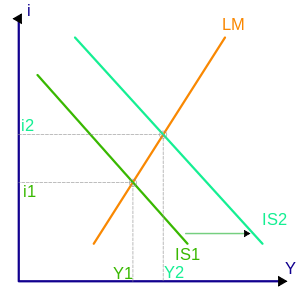
One hypothesis is that a government's deficit spending ("fiscal policy") has an effect similar to that of a lower saving rate or increased private fixed investment, increasing the amount of demand for goods at each individual interest rate. An increased deficit by the national government shifts the IS curve to the right. This raises the equilibrium interest rate (from i1 to i2) and national income (from Y1 to Y2), as shown in the graph above. The equilibrium level of national income in the IS-LM diagram is referred to as aggregate demand.
Keynesians argue spending may actually "crowd in" (encourage) private fixed investment via the accelerator effect, which helps long-term growth. Further, if government deficits are spent on productive public investment (e.g., infrastructure or public health) that spending directly and eventually raises potential output, although not necessarily more (or less) than the lost private investment might have. The extent of any crowding out depends on the shape of the LM curve. A shift in the IS curve along a relatively flat LM curve can increase output substantially with little change in the interest rate. On the other hand, an rightward shift in the IS curve along a vertical LM curve will lead to higher interest rates, but no change in output (this case represents the "treasury view").
Rightward shifts of the IS curve also result from exogenous increases in investment spending (i.e., for reasons other than interest rates or income), in consumer spending, and in export spending by people outside the economy being modelled, as well as by exogenous decreases in spending on imports. Thus these too raise both equilibrium income and the equilibrium interest rate. Of course, changes in these variables in the opposite direction shift the IS curve in the opposite direction.
The IS–LM model also allows for the role of monetary policy. If the money supply is increased, that shifts the LM curve downward or to the right, lowering interest rates and raising equilibrium national income. Further, exogenous decreases in liquidity preference, perhaps due to improved transactions technologies, lead to downward shifts of the LM curve and thus increases in income and decreases in interest rates. Changes in these variables in the opposite direction shift the LM curve in the opposite direction.
Incorporation into larger models
By itself, the IS–LM model is used to study the short run when prices are fixed or sticky and no inflation is taken into consideration. But in practice the main role of the model is as a sub-model of larger models (especially the Aggregate Demand-Aggregate Supply model – the AD–AS model) which allow for a flexible price level. In the aggregate demand-aggregate supply model, each point on the aggregate demand curve is an outcome of the IS–LM model for aggregate demand Y based on a particular price level. Starting from one point on the aggregate demand curve, at a particular price level and a quantity of aggregate demand implied by the IS–LM model for that price level, if one considers a higher potential price level, in the IS–LM model the real money supply M/P will be lower and hence the LM curve will be shifted higher, leading to lower aggregate demand; hence at the higher price level the level of aggregate demand is lower, so the aggregate demand curve is negatively sloped.
See also
References
- ↑ Gordon, Robert J. (2009). Macroeconomics (Eleventh ed.). Boston: Pearson Addison Wesley. ISBN 9780321552075.
- ↑ Mankiw, N. Gregory (2012). Macroeconomics (Eighth ed.). New York: Worth Publishers. ISBN 9781429240024.
- ↑ Sloman, John; Wride, Alison (2009). Economics (Seventh ed.). Prentice Hall. ISBN 9780273715627.
- 1 2 3 Hicks, J. R. (1937). "Mr. Keynes and the 'Classics': A Suggested Interpretation". Econometrica. 5 (2): 147–159. doi:10.2307/1907242.
- ↑ Hansen, A. H. (1953). A Guide to Keynes. New York: McGraw Hill.
- ↑ Bentolila, Samuel (2005). "Hicks–Hansen model". An Eponymous Dictionary of Economics: A Guide to Laws and Theorems Named after Economists. Edward Elgar. ISBN 1-84376-029-0.
- ↑ Colander, David (2004). "The Strange Persistence of the IS-LM Model" (PDF). History of Political Economy. 36 (Annual Supplement): 305–322. doi:10.1215/00182702-36-suppl_1-305.
- ↑ Meade, J. E. (1937). "A Simplified Model of Mr. Keynes' System". Review of Economic Studies. 4 (2): 98–107. JSTOR 2967607.
- 1 2 Hicks, John (1981). "'IS-LM': An Explanation". Journal of Post Keynesian Economics. 3 (2): 139–154. JSTOR 4537583.
- ↑ Mankiw, N. Gregory (May 2006). "The Macroeconomist as Scientist and Engineer" (PDF). p. 19. Retrieved 2014-11-17.
- ↑ Krugman, Paul Supply and Demand and QWERTY. February 8, 2011.
- ↑ Fonseca, Gonçalo L., The General Glut Controversy, The New School, archived from the original on 2003-07-26
Further reading
- Ackley, Gardner (1978). "The 'IS–LM' Form of the Model". Macroeconomics: Theory and Policy. New York: Macmillan. pp. 358–383. ISBN 0-02-300290-5.
- Barro, Robert J. (1984). "The Keynesian Theory of Business Fluctuations". Macroeconomics. New York: John Wiley. pp. 487–513. ISBN 0-471-87407-8.
- Darby, Michael R. (1976). "The Complete Keynesian Model". Macroeconomics. New York: McGraw-Hill. pp. 285–304. ISBN 0-07-015346-9.
- Dernburg, Thomas F.; McDougall, Duncan M. (1980). "Macroeconomic Equilibrium: The Level of Economic Activity". Macroeconomics (Sixth ed.). New York: McGraw-Hill. pp. 53–229. ISBN 0-07-016534-3.
- Keiser, Norman F. (1975). "The Real-Goods and Monetary Spheres". Macroeconomics (Second ed.). New York: Random House. pp. 231–260. ISBN 0-394-31922-2.
- Leijonhufvud, Axel (1983). "What is Wrong with IS/LM?". In Fitoussi, Jean-Paul. Modern Macroeconomic Theory. Oxford: Blackwell. pp. 49–90. ISBN 0-631-13158-2.
- Mankiw, N. Gregory (2013). "Aggregate Demand I+II". Macroeconomics (Eighth international ed.). London: Palgrave Macmillan. pp. 301–352. ISBN 978-1-4641-2167-8.
- Sawyer, John A. (1989). "A Model from Keynes's General Theory". Macroeconomic Theory. New York: Harvester Wheatsheaf. pp. 62–95. ISBN 0-7450-0555-1.
- Smith, Warren L. (1956). "A Graphical Exposition of the Complete Keynesian System". Southern Economic Journal. 23 (2): 115–125. doi:10.2307/1053551.
- Vroey, Michel de; Hoover, Kevin D., eds. (2004). The IS-LM model: Its Rise, Fall, and Strange Persistence. Durham: Duke University Press. ISBN 0-8223-6631-2.
- Young, Warren; Zilberfarb, Ben-Zion, eds. (2000). IS-LM and Modern Macroeconomics. Recent Economic Thought. 73. Springer Science & Business Media. ISBN 0-7923-7966-7.
External links
| Wikimedia Commons has media related to IS-LM model diagrams. |
- Krugman, Paul. There's something about macro – An explanation of the model and its role in understanding macroeconomics.
- Krugman, Paul. IS-LMentary – A basic explanation of the model and its uses.
- Wiens, Elmer G. IS–LM model – An online, interactive IS–LM model of the Canadian economy.