Hyperelastic material
| Continuum mechanics | ||||
|---|---|---|---|---|
 | ||||
|
Laws
|
||||
A hyperelastic or Green elastic material[1] is a type of constitutive model for ideally elastic material for which the stress-strain relationship derives from a strain energy density function. The hyperelastic material is a special case of a Cauchy elastic material.
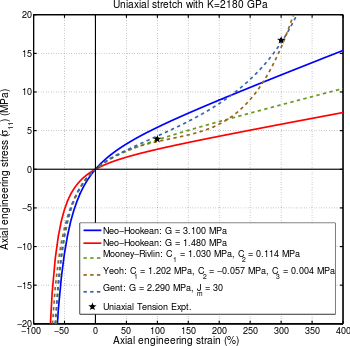
For many materials, linear elastic models do not accurately describe the observed material behaviour. The most common example of this kind of material is rubber, whose stress-strain relationship can be defined as non-linearly elastic, isotropic, incompressible and generally independent of strain rate. Hyperelasticity provides a means of modeling the stress-strain behavior of such materials.[2] The behavior of unfilled, vulcanized elastomers often conforms closely to the hyperelastic ideal. Filled elastomers and biological tissues are also often modeled via the hyperelastic idealization.
Ronald Rivlin and Melvin Mooney developed the first hyperelastic models, the Neo-Hookean and Mooney–Rivlin solids. Many other hyperelastic models have since been developed. Other widely used hyperelastic material models include the Ogden model and the Arruda–Boyce model.
Hyperelastic material models
Saint Venant–Kirchhoff model
The simplest hyperelastic material model is the Saint Venant–Kirchhoff model which is just an extension of the linear elastic material model to the nonlinear regime. This model has the form

where  is the second Piola–Kirchhoff stress and
  is the Lagrangian Green strain,
  and
and  are the Lamé constants, and
  is the second order unit tensor.
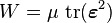
The strain-energy density function for the St. Venant–Kirchhoff model is
![W(\boldsymbol{E}) = \frac{\lambda}{2}[\text{tr}(\boldsymbol{E})]^2 + \mu \text{tr}(\boldsymbol{E}^2)](../I/m/d5b9114defd9892677205c0b564ce0f2.png)
and the second Piola–Kirchhoff stress can be derived from the relation

Classification of hyperelastic material models
Hyperelastic material models can be classified as:
1) phenomenological descriptions of observed behavior
- Fung
- Mooney–Rivlin
- Ogden
- Polynomial
- Saint Venant–Kirchhoff
- Yeoh
- Marlow
2) mechanistic models deriving from arguments about underlying structure of the material
3) hybrids of phenomenological and mechanistic models
- Gent
- Van der Waals
Generally, a hyperelastic model should satisfy the Drucker stability criterion.
Some hyperelastic models satisfy the Valanis-Landel hypothesis which states that the strain energy function can be separated into the sum of separate functions of the principal stretches  :
:

Stress-strain relations
Compressible hyperelastic materials
First Piola–Kirchhoff stress
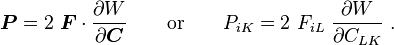
If  is the strain energy density function, the 1st Piola–Kirchhoff stress tensor can be calculated for a hyperelastic material as
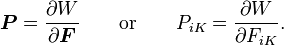
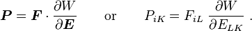
where  is the deformation gradient. In terms of the Lagrangian Green strain ()
In terms of the right Cauchy–Green deformation tensor ( )
)
Second Piola–Kirchhoff stress
If is the second Piola–Kirchhoff stress tensor then
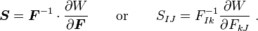
In terms of the Lagrangian Green strain
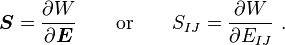
In terms of the right Cauchy–Green deformation tensor

The above relation is also known as the Doyle-Ericksen formula in the material configuration.
Cauchy stress
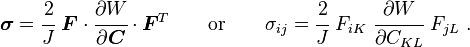
Similarly, the Cauchy stress is given by

In terms of the Lagrangian Green strain

In terms of the right Cauchy–Green deformation tensor
The above expressions are valid even for anisotropic media (in which case, the potential function is understood to depend implicitly on reference directional quantities such as initial fiber orientations). In the special case of isotropy, the Cauchy stress can be expressed in terms of the left Cauchy-Green deformation tensor as follows:[3]

Incompressible hyperelastic materials
For an incompressible material  . The incompressibility constraint is therefore
  . To ensure incompressibility of a hyperelastic material, the strain-energy function can be written in form:

where the hydrostatic pressure  functions as a Lagrangian multiplier to enforce the incompressibility constraint. The 1st Piola–Kirchhoff stress now becomes

This stress tensor can subsequently be converted into any of the other conventional stress tensors, such as the Cauchy Stress tensor which is given by

Expressions for the Cauchy stress
Compressible isotropic hyperelastic materials
For isotropic hyperelastic materials, the Cauchy stress can be expressed in terms of the invariants of the left Cauchy–Green deformation tensor (or right Cauchy–Green deformation tensor). If the strain energy density function is  , then
![\begin{align}
\boldsymbol{\sigma} & =
\cfrac{2}{\sqrt{I_3}}\left[\left(\cfrac{\partial\hat{W}}{\partial I_1} + I_1~\cfrac{\partial\hat{W}}{\partial I_2}\right)\boldsymbol{B} - \cfrac{\partial\hat{W}}{\partial I_2}~\boldsymbol{B} \cdot\boldsymbol{B} \right] + 2\sqrt{I_3}~\cfrac{\partial\hat{W}}{\partial I_3}~\boldsymbol{\mathit{1}} \\
& = \cfrac{2}{J}\left[\cfrac{1}{J^{2/3}}\left(\cfrac{\partial\bar{W}}{\partial \bar{I}_1} + \bar{I}_1~\cfrac{\partial\bar{W}}{\partial \bar{I}_2}\right)\boldsymbol{B} -
\cfrac{1}{J^{4/3}}~\cfrac{\partial\bar{W}}{\partial \bar{I}_2}~\boldsymbol{B} \cdot\boldsymbol{B} \right] \\
& \qquad \qquad + \left[\cfrac{\partial\bar{W}}{\partial J} - \cfrac{2}{3J}\left(\bar{I}_1~\cfrac{\partial\bar{W}}{\partial \bar{I}_1} + 2~\bar{I}_2~\cfrac{\partial\bar{W}}{\partial \bar{I}_2}\right)\right] ~\boldsymbol{\mathit{1}} \\
& = \cfrac{2}{J}\left[\left(\cfrac{\partial\bar{W}}{\partial \bar{I}_1} + \bar{I}_1~\cfrac{\partial\bar{W}}{\partial \bar{I}_2}\right)\bar{\boldsymbol{B}} -
\cfrac{\partial\bar{W}}{\partial \bar{I}_2}~\bar{\boldsymbol{B}} \cdot\bar{\boldsymbol{B}} \right] + \left[\cfrac{\partial\bar{W}}{\partial J} - \cfrac{2}{3J}\left(\bar{I}_1~\cfrac{\partial\bar{W}}{\partial \bar{I}_1} + 2~\bar{I}_2~\cfrac{\partial\bar{W}}{\partial \bar{I}_2}\right)\right] ~\boldsymbol{\mathit{1}} \\
& = \cfrac{\lambda_1}{\lambda_1\lambda_2\lambda_3}~\cfrac{\partial\tilde{W}}{\partial \lambda_1}~\mathbf{n}_1\otimes\mathbf{n}_1 + \cfrac{\lambda_2}{\lambda_1\lambda_2\lambda_3}~\cfrac{\partial\tilde{W}}{\partial \lambda_2}~\mathbf{n}_2\otimes\mathbf{n}_2 + \cfrac{\lambda_3}{\lambda_1\lambda_2\lambda_3}~\cfrac{\partial\tilde{W}}{\partial \lambda_3}~\mathbf{n}_3\otimes\mathbf{n}_3
\end{align}](../I/m/966b8f96a721450118f6bd9b76e51ff4.png)
(See the page on the left Cauchy–Green deformation tensor for the definitions of these symbols).
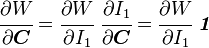
Proof 1: The second Piola–Kirchhoff stress tensor for a hyperelastic material is given by where
 is the right Cauchy–Green deformation tensor and is the deformation gradient. The Cauchy stress is given by
where
 . Let
. Let  be the three principal invariants of . Then
The derivatives of the invariants of the symmetric tensor
areTherefore, we can write
Plugging into the expression for the Cauchy stress gives
Using the left Cauchy–Green deformation tensor
 and noting that
  , we can write
For an incompressible material
 and hence
  .Then
.ThenTherefore, the Cauchy stress is given by
where
is an undetermined pressure which acts as a Lagrange multiplier to enforce the incompressibility constraint.If, in addition,
 , we have
  and hence
In that case the Cauchy stress can be expressed as
Proof 2: The isochoric deformation gradient is defined as  , resulting in the isochoric deformation gradient having a determinant of 1, in other words it is volume stretch free. Using this one can subsequently define the isochoric left Cauchy–Green deformation tensor tensor
  .
.
The invariants of
 are
are
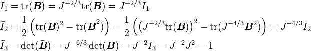 The set of invariants which are used to define the distortional behavior are the first two invariants of the isochoric left Cauchy–Green deformation tensor tensor, (which are identical to the ones for the right Cauchy Green stretch tensor), and add
  into the fray to describe the volumetric behaviour.
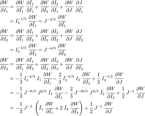
To express the Cauchy stress in terms of the invariants
 recall that
The chain rule of differentiation gives us
Recall that the Cauchy stress is given by
In terms of the invariants
we havePlugging in the expressions for the derivatives of
 in terms of , we have
or,
In terms of the deviatoric part of
 , we can write
For an incompressible material
 and hence
 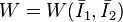 .Then
the Cauchy stress is given by
.Then
the Cauchy stress is given bywhere
is an undetermined pressure-like Lagrange multiplier term. In addition, if  , we have
  and hence
the Cauchy stress can be expressed as
and hence
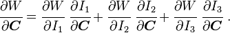
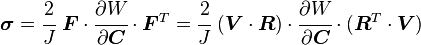
the Cauchy stress can be expressed asProof 3: To express the Cauchy stress in terms of the stretches  recall that
The chain rule gives
The Cauchy stress is given by
Plugging in the expression for the derivative of
leads toUsing the spectral decomposition of
 we have
Also note that
Therefore, the expression for the Cauchy stress can be written as
For an incompressible material
 and hence
 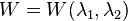 . Following Ogden[1] p. 485, we may write
Some care is to required at this stage because, when an eigenvalue is repeated, it is in general only Gâteaux differentiable, but not Fréchet differentiable.[4][5] A rigorous tensor derivative can only be found by solving another eigenvalue problem.
If we express the stress in terms of differences between components,
If in addition to incompressibility we have
 then a possible solution to the problem
requires
then a possible solution to the problem
requires  and we can write the stress differences as


![\boldsymbol{\sigma}
= \cfrac{2}{J}~\left[\cfrac{\partial W}{\partial I_1}~\boldsymbol{F}\cdot\boldsymbol{F}^T+
\cfrac{\partial W}{\partial I_2}~(I_1~\boldsymbol{F}\cdot\boldsymbol{F}^T - \boldsymbol{F}\cdot\boldsymbol{F}^T\cdot\boldsymbol{F}\cdot\boldsymbol{F}^T) +
\cfrac{\partial W}{\partial I_3}~I_3~\boldsymbol{\mathit{1}}\right]](../I/m/c91e47183342adeca48ec26635cc9b87.png)
![\boldsymbol{\sigma}
= \cfrac{2}{\sqrt{I_3}}~\left[\left(\cfrac{\partial W}{\partial I_1} +
I_1~\cfrac{\partial W}{\partial I_2}\right)~\boldsymbol{B} -
\cfrac{\partial W}{\partial I_2}~\boldsymbol{B}\cdot\boldsymbol{B}\right] +
2~\sqrt{I_3}~\cfrac{\partial W}{\partial I_3}~\boldsymbol{\mathit{1}}~.](../I/m/8decf07192533e05867d8c9d2ff0b260.png)

![\boldsymbol{\sigma}
= 2\left[\left(\cfrac{\partial W}{\partial I_1} +
I_1~\cfrac{\partial W}{\partial I_2}\right)~\boldsymbol{B} -
\cfrac{\partial W}{\partial I_2}~\boldsymbol{B}\cdot\boldsymbol{B}\right] - p~\boldsymbol{\mathit{1}}~.](../I/m/718f2033f987a31970e80ab9a65fd984.png)


![\boldsymbol{\sigma}
= \cfrac{2}{J}~\left[\left(\cfrac{\partial W}{\partial I_1}+
J^{2/3}~\bar{I}_1~\cfrac{\partial W}{\partial I_2}\right)~\boldsymbol{B} -
\cfrac{\partial W}{\partial I_2}~\boldsymbol{B}\cdot\boldsymbol{B}\right] +
2~J~\cfrac{\partial W}{\partial I_3}~\boldsymbol{\mathit{1}}~.](../I/m/0c6372c97d622040f61a8790627fcef8.png)
![\begin{align}
\boldsymbol{\sigma}
& = \cfrac{2}{J}~\left[\left(J^{-2/3}~\cfrac{\partial W}{\partial \bar{I}_1} +
J^{-2/3}~\bar{I}_1~\cfrac{\partial W}{\partial \bar{I}_2}\right)~\boldsymbol{B} -
J^{-4/3}~\cfrac{\partial W}{\partial \bar{I}_2}~\boldsymbol{B}\cdot\boldsymbol{B}\right]
+ \\
& \qquad
2~J~\left[-\cfrac{1}{3}~J^{-2}~\left(\bar{I}_1~\cfrac{\partial W}{\partial \bar{I}_1}+
2~\bar{I}_2~\cfrac{\partial W}{\partial \bar{I}_2}\right) +
\cfrac{1}{2}~J^{-1}~\cfrac{\partial W}{\partial J}\right]~\boldsymbol{\mathit{1}}
\end{align}](../I/m/fb798c6b10a2ea592718f8c9ddffc794.png)
![\begin{align}
\boldsymbol{\sigma}
& = \cfrac{2}{J}~\left[\cfrac{1}{J^{2/3}}~\left(\cfrac{\partial W}{\partial \bar{I}_1} +
\bar{I}_1~\cfrac{\partial W}{\partial \bar{I}_2}\right)~\boldsymbol{B} -
\cfrac{1}{J^{4/3}}~
\cfrac{\partial W}{\partial \bar{I}_2}~\boldsymbol{B}\cdot\boldsymbol{B}\right] \\
& \qquad + \left[\cfrac{\partial W}{\partial J} -
\cfrac{2}{3J}\left(\bar{I}_1~\cfrac{\partial W}{\partial \bar{I}_1}+
2~\bar{I}_2~\cfrac{\partial W}{\partial \bar{I}_2}\right)\right]\boldsymbol{\mathit{1}}
\end{align}](../I/m/e21a996463d22a12f2a1795527439605.png)
![\begin{align}
\boldsymbol{\sigma}
& = \cfrac{2}{J}~\left[\left(\cfrac{\partial W}{\partial \bar{I}_1} +
\bar{I}_1~\cfrac{\partial W}{\partial \bar{I}_2}\right)~\bar{\boldsymbol{B}} -
\cfrac{\partial W}{\partial \bar{I}_2}~\bar{\boldsymbol{B}}\cdot\bar{\boldsymbol{B}}\right] \\
& \qquad + \left[\cfrac{\partial W}{\partial J} -
\cfrac{2}{3J}\left(\bar{I}_1~\cfrac{\partial W}{\partial \bar{I}_1}+
2~\bar{I}_2~\cfrac{\partial W}{\partial \bar{I}_2}\right)\right]\boldsymbol{\mathit{1}}
\end{align}](../I/m/94354e87d33981379dff78e817a40647.png)
![\boldsymbol{\sigma}
= 2\left[\left(\cfrac{\partial W}{\partial \bar{I}_1} +
I_1~\cfrac{\partial W}{\partial \bar{I}_2}\right)~\bar{\boldsymbol{B}} -
\cfrac{\partial W}{\partial \bar{I}_2}~\bar{\boldsymbol{B}}\cdot\bar{\boldsymbol{B}}\right] - p~\boldsymbol{\mathit{1}}~.](../I/m/502d3c2d1e43dda51c3d6e29db972f24.png)
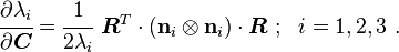
![\begin{align}
\cfrac{\partial W}{\partial\boldsymbol{C}} & =
\cfrac{\partial W}{\partial \lambda_1}~\cfrac{\partial \lambda_1}{\partial\boldsymbol{C}} +
\cfrac{\partial W}{\partial \lambda_2}~\cfrac{\partial \lambda_2}{\partial\boldsymbol{C}} +
\cfrac{\partial W}{\partial \lambda_3}~\cfrac{\partial \lambda_3}{\partial\boldsymbol{C}} \\
& = \boldsymbol{R}^T\cdot\left[\cfrac{1}{2\lambda_1}~\cfrac{\partial W}{\partial \lambda_1}~\mathbf{n}_1\otimes\mathbf{n}_1 +
\cfrac{1}{2\lambda_2}~\cfrac{\partial W}{\partial \lambda_2}~\mathbf{n}_2\otimes\mathbf{n}_2 +
\cfrac{1}{2\lambda_3}~\cfrac{\partial W}{\partial \lambda_3}~\mathbf{n}_3\otimes\mathbf{n}_3\right]\cdot\boldsymbol{R}
\end{align}](../I/m/2631a5e8c649a47ff677d53584b9f832.png)
![\boldsymbol{\sigma} =
\cfrac{2}{J}~\boldsymbol{V}\cdot
\left[\cfrac{1}{2\lambda_1}~
\cfrac{\partial W}{\partial \lambda_1}~\mathbf{n}_1\otimes\mathbf{n}_1 +
\cfrac{1}{2\lambda_2}~
\cfrac{\partial W}{\partial \lambda_2}~\mathbf{n}_2\otimes\mathbf{n}_2 +
\cfrac{1}{2\lambda_3}~
\cfrac{\partial W}{\partial \lambda_3}~\mathbf{n}_3\otimes\mathbf{n}_3\right]
\cdot\boldsymbol{V}](../I/m/8615d6f5397b96590bd29453c836c5d7.png)


![\boldsymbol{\sigma} =
\cfrac{1}{\lambda_1\lambda_2\lambda_3}~
\left[\lambda_1~\cfrac{\partial W}{\partial \lambda_1}~\mathbf{n}_1\otimes\mathbf{n}_1 +
\lambda_2~\cfrac{\partial W}{\partial \lambda_2}~\mathbf{n}_2\otimes\mathbf{n}_2 +
\lambda_3~\cfrac{\partial W}{\partial \lambda_3}~\mathbf{n}_3\otimes\mathbf{n}_3
\right]](../I/m/06ca5deb640339a232dcd26e3e3357ee.png)


Incompressible isotropic hyperelastic materials
For incompressible isotropic hyperelastic materials, the strain energy density function is 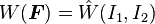 . The Cauchy stress is then given by
![\begin{align}
\boldsymbol{\sigma} & = -p~\boldsymbol{\mathit{1}} +
2\left[\left(\cfrac{\partial\hat{W}}{\partial I_1} + I_1~\cfrac{\partial\hat{W}}{\partial I_2}\right)\boldsymbol{B} - \cfrac{\partial\hat{W}}{\partial I_2}~\boldsymbol{B} \cdot\boldsymbol{B} \right] \\
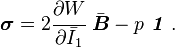
& = - p~\boldsymbol{\mathit{1}} + 2\left[\left(\cfrac{\partial W}{\partial \bar{I}_1} +
I_1~\cfrac{\partial W}{\partial \bar{I}_2}\right)~\bar{\boldsymbol{B}} -
\cfrac{\partial W}{\partial \bar{I}_2}~\bar{\boldsymbol{B}}\cdot\bar{\boldsymbol{B}}\right] \\
& = - p~\boldsymbol{\mathit{1}} + \lambda_1~\cfrac{\partial W}{\partial \lambda_1}~\mathbf{n}_1\otimes\mathbf{n}_1 +
\lambda_2~\cfrac{\partial W}{\partial \lambda_2}~\mathbf{n}_2\otimes\mathbf{n}_2 + \lambda_3~\cfrac{\partial W}{\partial \lambda_3}~\mathbf{n}_3\otimes\mathbf{n}_3
\end{align}](../I/m/faac2728ae4bd017490351fff2dccc61.png)
where is an undetermined pressure. In terms of stress differences
If in addition , then
If , then
Consistency with linear elasticity
Consistency with linear elasticity is often used to determine some of the parameters of hyperelastic material models. These consistency conditions can be found by comparing Hooke's law with linearized hyperelasticity at small strains.
Consistency conditions for isotropic hyperelastic models
For isotropic hyperelastic materials to be consistent with isotropic linear elasticity, the stress-strain relation should have the following form in the infinitesimal strain limit:

where  are the Lame constants. The strain energy density function that corresponds to the above relation is[1]
![W = \tfrac{1}{2}\lambda~[\mathrm{tr}(\boldsymbol{\varepsilon})]^2 + \mu~\mathrm{tr}(\boldsymbol{\varepsilon}^2)](../I/m/ab48a1c6eb39b1c83d1be4a149deaed2.png)
For an incompressible material  and we have
For any strain energy density function 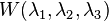 to reduce to the above forms for small strains the following conditions have to be met[1]
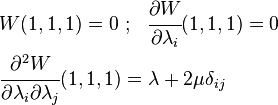
If the material is incompressible, then the above conditions may be expressed in the following form.
These conditions can be used to find relations between the parameters of a given hyperelastic model and shear and bulk moduli.
Consistency conditions for incompressible  based rubber materials
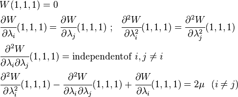
Many elastomers are modeled adequately by a strain energy density function that depends only on . For such materials we have .
The consistency conditions for incompressible materials for  may then be expressed as
The second consistency condition above can be derived by noting that

The can then be substituted into the consistency condition for isotropic incompressible hyperelastic materials.
References
- 1 2 3 4 R.W. Ogden, 1984, Non-Linear Elastic Deformations, ISBN 0-486-69648-0, Dover.
- ↑ Muhr, A. H. (2005). Modeling the stress-strain behavior of rubber. Rubber chemistry and technology, 78(3), 391-425.
- ↑ Y. Basar, 2000, Nonlinear continuum mechanics of solids, Springer, p. 157.
- ↑ Fox & Kapoor, Rates of change of eigenvalues and eigenvectors, AIAA Journal, 6 (12) 2426–2429 (1968)
- ↑ Friswell MI. The derivatives of repeated eigenvalues and their associated eigenvectors. Journal of Vibration and Acoustics (ASME) 1996; 118:390–397.
See also
- Cauchy elastic material
- Continuum mechanics
- Deformation (mechanics)
- Finite strain theory
- Rubber elasticity
- Stress measures
- Stress (mechanics)