Heteroscedasticity
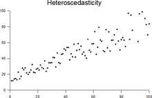
In statistics, a collection of random variables is heteroscedastic (or heteroskedastic;[notes 1] from Ancient Greek hetero “different” and skedasis “dispersion”) if there are sub-populations that have different variabilities from others. Here "variability" could be quantified by the variance or any other measure of statistical dispersion. Thus heteroscedasticity is the absence of homoscedasticity.
The existence of heteroscedasticity is a major concern in the application of regression analysis, including the analysis of variance, as it can invalidate statistical tests of significance that assume that the modelling errors are uncorrelated and uniform—hence that their variances do not vary with the effects being modeled. For instance, while the ordinary least squares estimator is still unbiased in the presence of heteroscedasticity, it is inefficient because the true variance and covariance are underestimated.[1][2] Similarly, in testing for differences between sub-populations using a location test, some standard tests assume that variances within groups are equal.
Because heteroscedasticity concerns expectations of the second moment of the errors, its presence is referred to as misspecification of the second order.[3]
Definition
Suppose there is a sequence of random variables and a sequence of vectors of random variables, . In dealing with conditional expectations of Yt given Xt, the sequence {Yt}t=1n is said to be heteroscedastic if the conditional variance of Yt given Xt, changes with t. Some authors refer to this as conditional heteroscedasticity to emphasize the fact that it is the sequence of conditional variances that changes and not the unconditional variance. In fact, it is possible to observe conditional heteroscedasticity even when dealing with a sequence of unconditional homoscedastic random variables; however, the opposite does not hold. If the variance changes only because of changes in value of X and not because of a dependence on the index t, the changing variance might be described using a scedastic function.


When using some statistical techniques, such as ordinary least squares (OLS), a number of assumptions are typically made. One of these is that the error term has a constant variance. This might not be true even if the error term is assumed to be drawn from identical distributions.
For example, the error term could vary or increase with each observation, something that is often the case with cross-sectional or time series measurements. Heteroscedasticity is often studied as part of econometrics, which frequently deals with data exhibiting it. While the influential 1980 paper by Halbert White used the term "heteroskedasticity" rather than "heteroscedasticity",[4] the latter spelling has been employed more frequently in later works.[5]
The econometrician Robert Engle won the 2003 Nobel Memorial Prize for Economics for his studies on regression analysis in the presence of heteroscedasticity, which led to his formulation of the autoregressive conditional heteroscedasticity (ARCH) modeling technique.
Consequences
One of the assumptions of the classical linear regression model is that there is no heteroscedasticity. Breaking this assumption means that the Gauss–Markov theorem does not apply, meaning that OLS estimators are not the Best Linear Unbiased Estimators (BLUE) and their variance is not the lowest of all other unbiased estimators. Heteroscedasticity does not cause ordinary least squares coefficient estimates to be biased, although it can cause ordinary least squares estimates of the variance (and, thus, standard errors) of the coefficients to be biased, possibly above or below the true or population variance. Thus, regression analysis using heteroscedastic data will still provide an unbiased estimate for the relationship between the predictor variable and the outcome, but standard errors and therefore inferences obtained from data analysis are suspect. Biased standard errors lead to biased inference, so results of hypothesis tests are possibly wrong. For example, if OLS is performed on a heteroscedastic data set, yielding biased standard error estimation, a researcher might fail to reject a null hypothesis at a given significance level, when that null hypothesis was actually uncharacteristic of the actual population (making a type II error).
Under certain assumptions, the OLS estimator has a normal asymptotic distribution when properly normalized and centered (even when the data does not come from a normal distribution). This result is used to justify using a normal distribution, or a chi square distribution (depending on how the test statistic is calculated), when conducting a hypothesis test. This holds even under heteroscedasticity. More precisely, the OLS estimator in the presence of heteroscedasticity is asymptotically normal, when properly normalized and centered, with a variance-covariance matrix that differs from the case of homoscedasticity. In 1980, White proposed a consistent estimator for the variance-covariance matrix of the asymptotic distribution of the OLS estimator.[4] This validates the use of hypothesis testing using OLS estimators and White's variance-covariance estimator under heteroscedasticity.
Heteroscedasticity is also a major practical issue encountered in ANOVA problems.[6] The F test can still be used in some circumstances.[7]
However, it has been said that students in econometrics should not overreact to heteroscedasticity.[5] One author wrote, "unequal error variance is worth correcting only when the problem is severe."[8] In addition, another word of caution was in the form, "heteroscedasticity has never been a reason to throw out an otherwise good model."[5][9] With the advent of heteroscedasticity-consistent standard errors allowing for inference without specifying the conditional second moment of error term, testing conditional homoscedasticity is not as important as in the past.
For any non-linear model (for instance Logit and Probit models), however, heteroscedasticity has more severe consequences: the maximum likelihood estimates of the parameters will be biased (in an unknown direction), as well as inconsistent (unless the likelihood function is modified to correctly take into account the precise form of heteroskedasticity).[10] As pointed out by Greene, “simply computing a robust covariance matrix for an otherwise inconsistent estimator does not give it redemption. Consequently, the virtue of a robust covariance matrix in this setting is unclear.”[11]
Detection
There are several methods to test for the presence of heteroscedasticity. Although tests for heteroscedasticity between groups can formally be considered as a special case of testing within regression models, some tests have structures specific to this case.
- Tests in regression
- Levene's test
- Goldfeld–Quandt test
- Park test[12]
- Glejser test[13][14]
- Brown–Forsythe test
- Harrison–McCabe test
- Breusch–Pagan test
- White test[4]
- Cook–Weisberg test
- Tests for grouped data
These tests consist of a test statistic (a mathematical expression yielding a numerical value as a function of the data), a hypothesis that is going to be tested (the null hypothesis), an alternative hypothesis, and a statement about the distribution of statistic under the null hypothesis.
Many introductory statistics and econometrics books, for pedagogical reasons, present these tests under the assumption that the data set in hand comes from a normal distribution. A great misconception is the thought that this assumption is necessary. Most of the methods of detecting heteroscedasticity outlined above can be modified for use even when the data do not come from a normal distribution. In many cases, this assumption can be relaxed, yielding a test procedure based on the same or similar test statistics but with the distribution under the null hypothesis evaluated by alternative routes: for example, by using asymptotic distributions which can be obtained from asymptotic theory, or by using resampling.
Fixes
There are four common corrections for heteroscedasticity. They are:
- View logarithmized data. Non-logarithmized series that are growing exponentially often appear to have increasing variability, random volatility, or volatility clusters as the series rises over time. The variability in percentage terms may, however, be rather stable. The reason for this is that the likelihood function for exponentially growing data lacks a variance. Using regression, the maximum likelihood estimator is the least squares estimator, a form of the sample mean, but the sampling distribution of the estimator is the Cauchy distribution. The Cauchy distribution has no variance and so there is no fixed point for the sample variance to converge to causing it to behave as a random number. Taking the logarithm of the data converts the likelihood function to the hyperbolic secant distribution, which has a defined variance.[15][16]
- Use a different specification for the model (different X variables, or perhaps non-linear transformations of the X variables).
- Apply a weighted least squares estimation method, in which OLS is applied to transformed or weighted values of X and Y. The weights vary over observations, usually depending on the changing error variances. In one variation the weights are directly related to the magnitude of the dependent variable, and this corresponds to least squares percentage regression.[17]
- Heteroscedasticity-consistent standard errors (HCSE), while still biased, improve upon OLS estimates.[4] HCSE is a consistent estimator of standard errors in regression models with heteroscedasticity. This method corrects for heteroscedasticity without altering the values of the coefficients. This method may be superior to regular OLS because if heteroscedasticity is present it corrects for it, however, if the data is homoscedastic, the standard errors are equivalent to conventional standard errors estimated by OLS. Several modifications of the White method of computing heteroscedasticity-consistent standard errors have been proposed as corrections with superior finite sample properties.
- Use MINQUE or even the customary estimators (for independent samples with observations each), whose efficiency losses are not substantial when the number of observations per sample is large (), especially for small number of independent samples.[18]


Examples
Heteroscedasticity often occurs when there is a large difference among the sizes of the observations.
- A classic example of heteroscedasticity is that of income versus expenditure on meals. As one's income increases, the variability of food consumption will increase. A poorer person will spend a rather constant amount by always eating inexpensive food; a wealthier person may occasionally buy inexpensive food and at other times eat expensive meals. Those with higher incomes display a greater variability of food consumption.
- Imagine you are watching a rocket take off nearby and measuring the distance it has traveled once each second. In the first couple of seconds your measurements may be accurate to the nearest centimeter, say. However, 5 minutes later as the rocket recedes into space, the accuracy of your measurements may only be good to 100 m, because of the increased distance, atmospheric distortion and a variety of other factors. The data you collect would exhibit heteroscedasticity.
Multivariate case
The study of heteroscedasticity has been generalized to the multivariate case, which deals with the covariances of vector observations instead of the variance of scalar observations. One version of this is to use covariance matrices as the multivariate measure of dispersion. Several authors have considered tests in this context, for both regression and grouped-data situations.[19][20] Bartlett's test for heteroscedasticity between grouped data, used most commonly in the univariate case, has also been extended for the multivariate case, but a tractable solution only exists for 2 groups.[21] Approximations exist for more than two groups, and they are both called Box's M test
Notes
- ↑ The spellings homoskedasticity and heteroskedasticity are also frequently used. Karl Pearson first used the word in 1905 with a c spelling.Pearson, Karl (1905). "Mathematical Contributions to the Theory of Evolution. XIV. On the General Theory of Skew Correlation and Non-linear Regression". Draper’s Company Research Memoirs: Biometric Series. II. J. Huston McCulloch argued that there should be a ‘k’ in the middle of the word and not a ‘c’. His argument was that the word had been constructed in English directly from Greek roots rather than coming into the English language indirectly via the French. See McCulloch, J. Huston (March 1985). "Miscellanea: On Heteros*edasticity". Econometrica. 53 (2): 483. JSTOR 1911250.
References
- ↑ Goldberger, Arthur S. (1964). Econometric Theory. New York: John Wiley & Sons. pp. 238–243.
- ↑ Johnston, J. (1972). Econometric Methods. New York: McGraw-Hill. pp. 214–221.
- ↑ Long, J. Scott; Trivedi, Pravin K. (1993). "Some Specification Tests for the Linear Regression Model". In Bollen, Kenneth A.; Long, J. Scott. Testing Structural Equation Models. London: Sage. pp. 66–110. ISBN 0-8039-4506-X.
- 1 2 3 4 White, Halbert (1980). "A heteroskedasticity-consistent covariance matrix estimator and a direct test for heteroskedasticity". Econometrica. 48 (4): 817–838. doi:10.2307/1912934. JSTOR 1912934.
- 1 2 3 Gujarati, D. N.; Porter, D. C. (2009). Basic Econometrics (Fifth ed.). Boston: McGraw-Hill Irwin. p. 400. ISBN 9780073375779.
- ↑ Jinadasa, Gamage; Weerahandi, Sam (1998). "Size performance of some tests in one-way anova". Communications in Statistics - Simulation and Computation. 27 (3): 625. doi:10.1080/03610919808813500.
- ↑ Bathke, A (2004). "The ANOVA F test can still be used in some balanced designs with unequal variances and nonnormal data". Journal of Statistical Planning and Inference. 126 (2): 413. doi:10.1016/j.jspi.2003.09.010.
- ↑ Fox, J. (1997). Applied Regression Analysis, Linear Models, and Related Methods. California: Sage Publications. p. 306. (Cited in Gujarati et al. 2009, p. 400)
- ↑ Mankiw, N. G. (1990). "A Quick Refresher Course in Macroeconomics". Journal of Economic Literature. 28 (4): 1645–1660 [p. 1648]. doi:10.3386/w3256. JSTOR 2727441.
- ↑ Giles, Dave (May 8, 2013). "Robust Standard Errors for Nonlinear Models". Econometrics Beat.
- ↑ Greene, William H. (2012). "Estimation and Inference in Binary Choice Models". Econometric Analysis (Seventh ed.). Boston: Pearson Education. pp. 730–755 [p. 733]. ISBN 978-0-273-75356-8.
- ↑ R. E. Park (1966). "Estimation with Heteroscedastic Error Terms". Econometrica. 34 (4): 888. doi:10.2307/1910108. JSTOR 1910108.
- ↑ Glejser, H. (1969). "A new test for heteroscedasticity". Journal of the American Statistical Association. 64 (325): 316–323. doi:10.1080/01621459.1969.10500976.
- ↑ Machado, José A. F.; Silva, J. M. C. Santos (2000). "Glejser's test revisited". Journal of Econometrics. 97 (1): 189–202. doi:10.1016/S0304-4076(00)00016-6.
- ↑ Mann, HB and Wald, A (1943). "On the Statistical Treatment of Linear Stochastic Difference Equations". Econometrica. 11: 173–200. doi:10.2307/1905674.
- ↑ White, John S. (1958). "The Limiting Distribution of the Serial Correlation Coefficient in the Explosive Case". 29: 1188–1197. doi:10.1214/aoms/1177706450.
- ↑ Tofallis, C (2008). "Least Squares Percentage Regression". Journal of Modern Applied Statistical Methods. 7: 526–534. doi:10.2139/ssrn.1406472. SSRN 1406472
 .
. - ↑ J. N. K. Rao (March 1973). "On the Estimation of Heteroscedastic Variances". Biometrics. 29 (1): 11–24. doi:10.2307/2529672. JSTOR 2529672.
- ↑ Holgersson, H. E. T.; Shukur, G. (2004). "Testing for multivariate heteroscedasticity". Journal of Statistical Computation and Simulation. 74 (12): 879. doi:10.1080/00949650410001646979.
- ↑ Gupta, A. K.; Tang, J. (1984). "Distribution of likelihood ratio statistic for testing equality of covariance matrices of multivariate Gaussian models". Biometrika. 71 (3): 555–559. doi:10.1093/biomet/71.3.555. JSTOR 2336564.
- ↑ d'Agostino, R. B.; Russell, H. K. (2005). "Multivariate Bartlett Test". Encyclopedia of Biostatistics. doi:10.1002/0470011815.b2a13048. ISBN 047084907X.
Further reading
Most statistics textbooks will include at least some material on heteroscedasticity. Some examples are:
- Asteriou, Dimitros; Hall, Stephen G. (2011). Applied Econometrics (Second ed.). Palgrave MacMillan. pp. 109–147. ISBN 978-0-230-27182-1.
- Davidson, Russell; MacKinnon, James G. (1993). Estimation and Inference in Econometrics. New York: Oxford University Press. pp. 547–582. ISBN 0-19-506011-3.
- Dougherty, Christopher (2011). Introduction to Econometrics. New York: Oxford University Press. pp. 280–299. ISBN 978-0-19-956708-9.
- Gujarati, Damodar N.; Porter, Dawn C. (2009). Basic Econometrics (Fifth ed.). New York: McGraw-Hill Irwin. pp. 365–411. ISBN 978-0-07-337577-9.
- Kmenta, Jan (1986). Elements of Econometrics (Second ed.). New York: Macmillan. pp. 269–298. ISBN 0-02-365070-2.
- Maddala, G. S.; Lahiri, Kajal (2009). Introduction to Econometrics (Fourth ed.). New York: Wiley. pp. 211–238. ISBN 978-0-470-01512-4.
External links
| |||||||||||||||||||||||||||||||||||||||||||||
| |||||||||||||||||||||||||||||||||||||||||||||
| |||||||||||||||||||||||||||||||||||||||||||||
| |||||||||||||||||||||||||||||||||||||||||||||
| |||||||||||||||||||||||||||||||||||||||||||||
| |||||||||||||||||||||||||||||||||||||||||||||
| |||||||||||||||||||||||||||||||||||||||||||||