Gram–Schmidt process

In mathematics, particularly linear algebra and numerical analysis, the Gram–Schmidt process is a method for orthonormalising a set of vectors in an inner product space, most commonly the Euclidean space Rn equipped with the standard inner product. The Gram–Schmidt process takes a finite, linearly independent set S = {v1, ..., vk} for k ≤ n and generates an orthogonal set S′ = {u1, ..., uk} that spans the same k-dimensional subspace of Rn as S.
The method is named after Jørgen Pedersen Gram and Erhard Schmidt but it appeared earlier in the work of Laplace and Cauchy. In the theory of Lie group decompositions it is generalized by the Iwasawa decomposition.[1]
The application of the Gram–Schmidt process to the column vectors of a full column rank matrix yields the QR decomposition (it is decomposed into an orthogonal and a triangular matrix).
The Gram–Schmidt process
We define the projection operator by

where denotes the inner product of the vectors v and u. This operator projects the vector v orthogonally onto the line spanned by vector u. If u = 0, we define . i.e., the projection map is the zero map, sending every vector to the zero vector.


The Gram–Schmidt process then works as follows:

The sequence u1, ..., uk is the required system of orthogonal vectors, and the normalized vectors e1, ..., ek form an orthonormal set. The calculation of the sequence u1, ..., uk is known as Gram–Schmidt orthogonalization, while the calculation of the sequence e1, ..., ek is known as Gram–Schmidt orthonormalization as the vectors are normalized.
To check that these formulas yield an orthogonal sequence, first compute ‹ u1,u2 › by substituting the above formula for u2: we get zero. Then use this to compute ‹ u1,u3 › again by substituting the formula for u3: we get zero. The general proof proceeds by mathematical induction.
Geometrically, this method proceeds as follows: to compute ui, it projects vi orthogonally onto the subspace U generated by u1, ..., ui−1, which is the same as the subspace generated by v1, ..., vi−1. The vector ui is then defined to be the difference between vi and this projection, guaranteed to be orthogonal to all of the vectors in the subspace U.
The Gram–Schmidt process also applies to a linearly independent countably infinite sequence {vi}i. The result is an orthogonal (or orthonormal) sequence {ui}i such that for natural number n: the algebraic span of v1, ..., vn is the same as that of u1, ..., un.
If the Gram–Schmidt process is applied to a linearly dependent sequence, it outputs the 0 vector on the ith step, assuming that vi is a linear combination of v1, ..., vi−1. If an orthonormal basis is to be produced, then the algorithm should test for zero vectors in the output and discard them because no multiple of a zero vector can have a length of 1. The number of vectors output by the algorithm will then be the dimension of the space spanned by the original inputs.
A variant of the Gram–Schmidt process using transfinite recursion applied to a (possibly uncountably) infinite sequence of vectors yields a set of orthonormal vectors with such that for any , the completion of the span of is the same as that of . In particular, when applied to a (algebraic) basis of a Hilbert space (or, more generally, a basis of any dense subspace), it yields a (functional-analytic) orthonormal basis. Note that in the general case often the strict inequality holds, even if the starting set was linearly independent, and the span of need not be a subspace of the span of (rather, it's a subspace of its completion).


Example
Consider the following set of vectors in R2 (with the conventional inner product)

Now, perform Gram–Schmidt, to obtain an orthogonal set of vectors:


We check that the vectors u1 and u2 are indeed orthogonal:

noting that if the dot product of two vectors is 0 then they are orthogonal.
For non-zero vectors, we can then normalize the vectors by dividing out their sizes as shown above:


Numerical stability
When this process is implemented on a computer, the vectors are often not quite orthogonal, due to rounding errors. For the Gram–Schmidt process as described above (sometimes referred to as "classical Gram–Schmidt") this loss of orthogonality is particularly bad; therefore, it is said that the (classical) Gram–Schmidt process is numerically unstable.

The Gram–Schmidt process can be stabilized by a small modification; this version is sometimes referred to as modified Gram-Schmidt or MGS. This approach gives the same result as the original formula in exact arithmetic and introduces smaller errors in finite-precision arithmetic. Instead of computing the vector uk as

it is computed as

Each step finds a vector orthogonal to . Thus is also orthogonalized against any errors introduced in computation of .


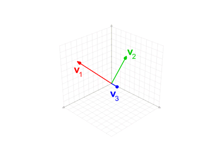
This method is used in the previous animation, when the intermediate v'3 vector is used when orthogonalizing the blue vector v3.
Algorithm
The following algorithm implements the stabilized Gram–Schmidt orthonormalization. The vectors v1, ..., vk (columns of matrix V, so that V(:,j) is the jth vector) are replaced by orthonormal vectors (columns of U) which span the same subspace.
   n = size(V,1);
   k = size(V,2);
   U = zeros(n,k);
   U(:,1) = V(:,1)/sqrt(V(:,1)'*V(:,1));
   for i = 2:k
     U(:,i) = V(:,i);
     for j = 1:i-1
       U(:,i) = U(:,i) - ( U(:,i)'*U(:,j) )*U(:,j);
     end
     U(:,i) = U(:,i)/sqrt(U(:,i)'*U(:,i));
   end
The cost of this algorithm is asymptotically O(nk2) floating point operations, where n is the dimensionality of the vectors (Golub & Van Loan 1996, §5.2.8).
Determinant formula
The result of the Gram–Schmidt process may be expressed in a non-recursive formula using determinants.


where D 0=1 and, for j ≥ 1, D j is the Gram determinant

Note that the expression for uk is a "formal" determinant, i.e. the matrix contains both scalars and vectors; the meaning of this expression is defined to be the result of a cofactor expansion along the row of vectors.
The determinant formula for the Gram-Schmidt is computationally slower (exponentially slower) than the recursive algorithms described above; it is mainly of theoretical interest.
Alternatives
Other orthogonalization algorithms use Householder transformations or Givens rotations. The algorithms using Householder transformations are more stable than the stabilized Gram–Schmidt process. On the other hand, the Gram–Schmidt process produces the th orthogonalized vector after the th iteration, while orthogonalization using Householder reflections produces all the vectors only at the end. This makes only the Gram–Schmidt process applicable for iterative methods like the Arnoldi iteration.

Yet another alternative is motivated by the use of Cholesky decomposition for inverting the matrix of the normal equations in linear least squares. Let be a full column rank matrix, whose columns need to be orthogonalized. The matrix is Hermitian and positive definite, so it can be written as using the Cholesky decomposition. The lower triangular matrix with strictly positive diagonal entries is invertible. Then columns of the matrix are orthonormal and span the same subspace as the columns of the original matrix . The explicit use of the product makes the algorithm unstable, especially if the product's condition number is large. Nevertheless, this algorithm is used in practice and implemented in some software packages because of its high efficiency and simplicity.


In quantum mechanics there are several orthogonalization schemes with characteristics better suited for certain applications than original Gram–Schmidt. Nevertheless, it remains a popular and effective algorithm for even the largest electronic structure calculations. [2]
References
- ↑ Cheney, Ward; Kincaid, David (2009). Linear Algebra: Theory and Applications. Sudbury, Ma: Jones and Bartlett. pp. 544, 558. ISBN 978-0-7637-5020-6.
- ↑ Hasegawa, et al., First-principles calculations of electron states of a silicon nanowire with 100,000 atoms on the K computer. 2011
- Bau III, David; Trefethen, Lloyd N. (1997), Numerical linear algebra, Philadelphia: Society for Industrial and Applied Mathematics, ISBN 978-0-89871-361-9.
- Golub, Gene H.; Van Loan, Charles F. (1996), Matrix Computations (3rd ed.), Johns Hopkins, ISBN 978-0-8018-5414-9.
- Greub, Werner (1975), Linear Algebra (4th ed.), Springer.
- Soliverez, C. E.; Gagliano, E. (1985), "Orthonormalization on the plane: a geometric approach" (PDF), Mex. J. Phys., 31 (4): 743–758.
External links
- Hazewinkel, Michiel, ed. (2001), "Orthogonalization", Encyclopedia of Mathematics, Springer, ISBN 978-1-55608-010-4
- Harvey Mudd College Math Tutorial on the Gram-Schmidt algorithm
- Earliest known uses of some of the words of mathematics: G The entry "Gram-Schmidt orthogonalization" has some information and references on the origins of the method.
- Demos: Gram Schmidt process in plane and Gram Schmidt process in space
- Gram-Schmidt orthogonalization applet
- NAG Gram–Schmidt orthogonalization of n vectors of order m routine
- Proof: Raymond Puzio, Keenan Kidwell. "proof of Gram-Schmidt orthogonalization algorithm" (version 8). PlanetMath.org.