Spectral density
The power spectrum of a time series describes the distribution of power into frequency components composing that signal. According to Fourier analysis any physical signal can be decomposed into a number of discrete frequencies, or a spectrum of frequencies over a continuous range. The statistical average of a certain signal or sort of signal (including noise) as analyzed in terms of its frequency content, is called its spectrum.


When the energy of the signal is concentrated around a finite time interval, especially if its total energy is finite, one may compute the energy spectral density. More commonly used is the power spectral density (or simply power spectrum), which applies to signals existing over all time, or over a time period large enough (especially in relation to the duration of a measurement) that it could as well have been over an infinite time interval. The power spectral density (PSD) then refers to the spectral energy distribution that would be found per unit time, since the total energy of such a signal over all time would generally be infinite. Summation or integration of the spectral components yields the total power (for a physical process) or variance (in a statistical process), identical to what would be obtained by integrating over the time domain, as dictated by Parseval's theorem.

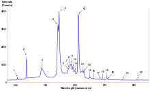
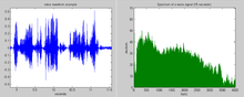
The spectrum of a physical process often contains essential information about the nature of . For instance, the pitch and timbre of a musical instrument are immediately determined from a spectral analysis. The color of a light source is determined by the spectrum of the electromagnetic wave's electric field as it fluctuates at an extremely high frequency. Obtaining a spectrum from time series such as these involves the Fourier transform, and generalizations based on Fourier analysis. In many cases the time domain is not specifically employed in practice, such as when a dispersive prism is used to obtain a spectrum of light in a spectrograph, or when a sound is perceived through its effect on the auditory receptors of the inner ear, each of which is sensitive to a particular frequency.


However this article concentrates on situations in which the time series is known (at least in a statistical sense) or directly measured (such as by a microphone sampled by a computer). The power spectrum is important in statistical signal processing and in the statistical study of stochastic processes, as well as in many other branches of physics and engineering. Typically the process is a function of time but one can similarly discuss data in the spatial domain being decomposed in terms of spatial frequency.
Explanation
Any signal that can be represented as an amplitude that varies in time has a corresponding frequency spectrum. This includes familiar entities such as visible light (perceived as color), musical notes (perceived as pitch), radio/TV (specified by their frequency, or sometimes wavelength) and even the regular rotation of the earth. When these signals are viewed in the form of a frequency spectrum, certain aspects of the received signals or the underlying processes producing them are revealed. In some cases the frequency spectrum may include a distinct peak corresponding to a sine wave component. And additionally there may be peaks corresponding to harmonics of a fundamental peak, indicating a periodic signal which is not simply sinusoidal. Or a continuous spectrum may show narrow frequency intervals which are strongly enhanced corresponding to resonances, or frequency intervals containing almost zero power as would be produced by a notch filter.
In physics, the signal might be a wave, such as an electromagnetic wave, an acoustic wave, or the vibration of a mechanism. The power spectral density (PSD) of the signal describes the power present in the signal as a function of frequency, per unit frequency. Power spectral density is commonly expressed in watts per hertz (W/Hz).[1]
When a signal is defined in terms only of a voltage, for instance, there is no unique power associated with the stated amplitude. In this case "power" is simply reckoned in terms of the square of the signal, as this would always be proportional to the actual power delivered by that signal into a given impedance. So one might use units of V2 Hz−1 for the PSD and V2 s Hz−1 for the ESD (energy spectral density)[2] even though no actual "power" or "energy" is specified.
Sometimes one encounters an amplitude spectral density (ASD), which is the square root of the PSD; the ASD of a voltage signal has units of V Hz−1/2.[3] This is useful when the shape of the spectrum is rather constant, since variations in the ASD will then be proportional to variations in the signal's voltage level itself. But it is mathematically preferred to use the PSD, since only in that case is the area under the curve meaningful in terms of actual power over all frequency or over a specified bandwidth.
For random vibration analysis, units of g2 Hz−1 are frequently used for the PSD of acceleration. Here g denotes the g-force.[4]
Mathematically it is not necessary to assign physical dimensions to the signal or to the independent variable. In the following discussion the meaning of x(t) will remain unspecified, but the independent variable will be assumed to be that of time.
Definition
Energy spectral density
Energy spectral density describes how the energy of a signal or a time series is distributed with frequency. Here, the term energy is used in the generalized sense of signal processing;[5] that is, the energy of a signal is


The energy spectral density is most suitable for transients—that is, pulse-like signals—having a finite total energy. In this case, Parseval's theorem [6] gives us an alternate expression for the energy of the signal in terms of its Fourier transform,


Here is the frequency in Hz, i.e., cycles per second. Often used is the angular frequency . Since the integral on the right-hand side is the energy of the signal, the integrand can be interpreted as a density function describing the energy per unit frequency contained in the signal at the frequency . In light of this, the energy spectral density of a signal is defined as[6]


As a physical example of how one might measure the energy spectral density of a signal, suppose represents the potential (in volts) of an electrical pulse propagating along a transmission line of impedance , and suppose the line is terminated with a matched resistor (so that all of the pulse energy is delivered to the resistor and none is reflected back). By Ohm's law, the power delivered to the resistor at time is equal to , so the total energy is found by integrating with respect to time over the duration of the pulse. To find the value of the energy spectral density at frequency , one could insert between the transmission line and the resistor a bandpass filter which passes only a narrow range of frequencies (, say) near the frequency of interest and then measure the total energy dissipated across the resistor. The value of the energy spectral density at is then estimated to be . In this example, since the power has units of V2 Ω−1, the energy has units of V2 s Ω−1 = J, and hence the estimate of the energy spectral density has units of J Hz−1, as required. In many situations, it is common to forgo the step of dividing by so that the energy spectral density instead has units of V2 s Hz−1.


This definition generalizes in a straightforward manner to a discrete signal with an infinite number of values such as a signal sampled at discrete times :


where is the discrete Fourier transform of and is the complex conjugate of . The sampling interval is needed to keep the correct physical units and to ensure that we recover the continuous case in the limit ; however, in the mathematical sciences, the interval is often set to 1.


Power spectral density
The above definition of energy spectral density is suitable for transients (pulse-like signals) whose energy is concentrated around one time window; then the Fourier transforms of the signals generally exist. For continuous signals over all time, such as stationary processes, one must rather define the power spectral density (PSD); this describes how power of a signal or time series is distributed over frequency, as in the simple example given previously. Here, power can be the actual physical power, or more often, for convenience with abstract signals, is simply identified with the squared value of the signal. For example, statisticians study the variance of a function over time x(t) (or over another independent variable), and using an analogy with electrical signals (among other physical processes), it is customary to refer to it as the power spectrum even when there is no physical power involved. If one were to create a physical voltage source which followed x(t) and applied it to the terminals of a 1 ohm resistor, then indeed the instantaneous power dissipated in that resistor would be given by x2 watts.
The average power P of a signal over all time is therefore given by the following time average:

Note that a stationary process, for instance, may have a finite power but an infinite energy. After all, energy is the integral of power, and the stationary signal continues over an infinite time. That is the reason that we cannot use the energy spectral density as defined above in such cases.
In analyzing the frequency content of the signal , one might like to compute the ordinary Fourier transform ; however, for many signals of interest the Fourier transform does not formally exist.[N 1] Because of this complication one can as well work with a truncated Fourier transform , where the signal is integrated only over a finite interval [0, T]:


Then the power spectral density can be defined as[8][9]
![S_{xx}(\omega )=\lim _{T\rightarrow \infty }\mathbf {E} \left[|{\hat {x}}_{T}(\omega )|^{2}\right].](../I/m/5e312ec8651b10b75551e5886eae747ff10fdaaf.svg)
Here E denotes the expected value; explicitly, we have[9]
![\mathbf {E} \left[|{\hat {x}}_{T}(\omega )|^{2}\right]=\mathbf {E} \left[{\frac {1}{T}}\int \limits _{0}^{T}x^{*}(t)e^{i\omega t}\,dt\int \limits _{0}^{T}x(t')e^{-i\omega t'}\,dt'\right]={\frac {1}{T}}\int \limits _{0}^{T}\int \limits _{0}^{T}\mathbf {E} \left[x^{*}(t)x(t')\right]e^{i\omega (t-t')}\,dt\,dt'.](../I/m/edfda400647431e434b9ba37e1d3606621d64c7d.svg)
In the latter form (for a stationary random process), one can make the change of variables and with the limits of integration (rather than [0,T]) approaching infinity, the resulting power spectral density and the autocorrelation function of this signal are seen to be Fourier transform pairs (Wiener–Khinchin theorem). The autocorrelation function is a statistic defined as (or more generally as in the case that X(t) is complex-valued). Provided that is absolutely integrable (which is not always true)[10],


Many authors use this equality to actually define the power spectral density.[11]
The power of the signal in a given frequency band (or ) can be calculated by integrating over frequency. Since , an equal amount of power can be attributed to positive and negative frequencies, which accounts for the factor of 2 in the following form (such trivial factors dependent on conventions used):
![[f_{1},f_{2}]](../I/m/1ce110719ca89eeeac9a2786c1fce4e86800dd41.svg)
![[\omega _{1},\omega _{2}]](../I/m/1dad129c74171365114e79fdd991264dda783b22.svg)


More generally, similar techniques may be used to estimate a time-varying spectral density. In this case the truncated Fourier transform defined above over the finite time interval (0, T) is not evaluated in the limit of T approaching infinity. This results in decreased spectral coverage and resolution since frequencies of less than 1/T are not sampled, and results at frequencies which are not an integer multiple of 1/T are not independent. Just using a single such time series, the estimated power spectrum will be very "noisy", however this can be alleviated if it is possible to evaluate the expected value (in the above equation) using a large (or infinite) number of short-term spectra corresponding to statistical ensembles of realizations of x(t) evaluated over the specified time window.
This definition of the power spectral density can be generalized to discrete time variables . As above we can consider a finite window of with the signal sampled at discrete times for a total measurement period . Then a single estimate of the PSD can be obtained through summation rather than integration:


- .

As before, the actual PSD is achieved when N (and thus T) approach infinity and the expected value is formally applied. In a real-world application, one would typically average this single-measurement PSD over many trials to obtain a more accurate estimate of the theoretical PSD of the physical process underlying the individual measurements. This computed PSD is sometimes called a periodogram. This periodogram converges to the true PSD as the number of estimates as well as the averaging time interval T approach infinity (Brown & Hwang[12]).
If two signals both possess power spectral densities, then the cross-spectral density can similarly be calculated; as the PSD is related to the autocorrelation, so is the cross-spectral density related to the cross-correlation.
Properties of the power spectral density
Some properties of the PSD include:[13]
- The spectrum of a real valued process (or even a complex process using the above definition) is real and an even function of frequency: .
- If the process is continuous and purely indeterministic, the autocovariance function can be reconstructed by using the Inverse Fourier transform
- The PSD can be used to compute the variance (net power) of a process by integrating over frequency:
- Being based on the fourier transform, the PSD is a linear function of the autocovariance function in the sense that if is decomposed into two functions , then


The integrated spectrum or power spectral distribution is defined as[14]


Cross-spectral density
Given two signals and , each of which possess power spectral densities and , it is possible to define a cross-spectral density (CSD) given by


![S_{xy}(\omega )=\lim _{T\rightarrow \infty }\mathbf {E} \left\{\left[F_{x}^{T}(\omega )\right]^{*}F_{y}^{T}(\omega )\right\}.](../I/m/b8c1472d73a681c8b15487334f5c8292edbb4d54.svg)
The cross-spectral density (or 'cross power spectrum') is thus the Fourier transform of the cross-correlation function.
![S_{xy}(\omega )=\int _{-\infty }^{\infty }R_{xy}(t)e^{-j\omega t}dt=\int _{-\infty }^{\infty }\left[\int _{-\infty }^{\infty }x(\tau )\cdot y(\tau +t)d\tau \right]\,e^{-j\omega t}dt,](../I/m/e2b65fae9851833f50e2ea10b02c6f9c191e3863.svg)
where is the cross-correlation of and .

By an extension of the Wiener–Khinchin theorem, the Fourier transform of the cross-spectral density is the cross-covariance function.[15] In light of this, the PSD is seen to be a special case of the CSD for .


For discrete signals xn and yn, the relationship between the cross-spectral density and the cross-covariance is

Estimation
The goal of spectral density estimation is to estimate the spectral density of a random signal from a sequence of time samples. Depending on what is known about the signal, estimation techniques can involve parametric or non-parametric approaches, and may be based on time-domain or frequency-domain analysis. For example, a common parametric technique involves fitting the observations to an autoregressive model. A common non-parametric technique is the periodogram.
The spectral density is usually estimated using Fourier transform methods (such as the Welch method), but other techniques such as the maximum entropy method can also be used.
Properties
- The spectral density of and the autocorrelation of form a Fourier transform pair (for PSD versus ESD, different definitions of autocorrelation function are used). This result is known as Wiener–Khinchin theorem.
- One of the results of Fourier analysis is Parseval's theorem which states that the area under the energy spectral density curve is equal to the area under the square of the magnitude of the signal, the total energy:


- The above theorem holds true in the discrete cases as well. A similar result holds for power: the area under the power spectral density curve is equal to the total signal power, which is , the autocorrelation function at zero lag. This is also (up to a constant which depends on the normalization factors chosen in the definitions employed) the variance of the data comprising the signal.

Related concepts
- The spectral centroid of a signal is the midpoint of its spectral density function, i.e. the frequency that divides the distribution into two equal parts.
- The spectral edge frequency of a signal is an extension of the previous concept to any proportion instead of two equal parts.
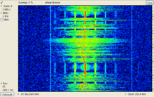
- The spectral density is a function of frequency, not a function of time. However, the spectral density of small windows of a longer signal may be calculated, and plotted versus time associated with the window. Such a graph is called a spectrogram. This is the basis of a number of spectral analysis techniques such as the short-time Fourier transform and wavelets.
- A "spectrum" generally means the power spectral density, as discussed above, which depicts the distribution of signal content over frequency. This is not to be confused with the frequency response of a transfer function which also includes a phase (or equivalently, a real and imaginary part as a function of frequency). For transfer functions, (e.g., Bode plot, chirp) the complete frequency response may be graphed in two parts, amplitude versus frequency and phase versus frequency (or less commonly, as real and imaginary parts of the transfer function). The impulse response (in the time domain) , cannot generally be uniquely recovered from the amplitude spectral density part alone without the phase function. Although these are also fourier transform pairs, there is no symmetry (as there is for the autocorrelation) forcing the fourier transform to be real-valued. See spectral phase and phase noise.

Applications
Electrical engineering
The concept and use of the power spectrum of a signal is fundamental in electrical engineering, especially in electronic communication systems, including radio communications, radars, and related systems, plus passive remote sensing technology. Electronic instruments called spectrum analyzers are used to observe and measure the power spectra of signals.
The spectrum analyzer measures the magnitude of the short-time Fourier transform (STFT) of an input signal. If the signal being analyzed can be considered a stationary process, the STFT is a good smoothed estimate of its power spectral density.
Cosmology
Primordial fluctuations, density variations in the early universe, are quantified by a power spectrum which gives the power of the variations as a function of spatial scale.
See also
- Coherence (signal processing), for use of the cross-spectral density.
- Noise spectral density
- Spectral density estimation
- Spectral efficiency
- Spectral power distribution
- Brightness temperature
- Colors of noise
- Spectral leakage
- Window function
- Bispectrum
- Whittle likelihood
Notes
- ↑ Some authors (e.g. Risken[7]
) still use the non-normalized Fourier transform in a formal way to formulate a definition of the power spectral density
- ,


References
- ↑ Gérard Maral (2003). VSAT Networks. John Wiley and Sons. ISBN 0-470-86684-5.
- ↑ Michael Peter Norton & Denis G. Karczub (2003). Fundamentals of Noise and Vibration Analysis for Engineers. Cambridge University Press. ISBN 0-521-49913-5.
- ↑ Michael Cerna & Audrey F. Harvey (2000). "The Fundamentals of FFT-Based Signal Analysis and Measurement" (PDF).
- ↑ Alessandro Birolini (2007). Reliability Engineering. Springer. p. 83. ISBN 978-3-540-49388-4.
- ↑ Oppenheim; Verghese. Signals, Systems, and Inference. pp. 32–4.
- 1 2 Stein, Jonathan Y. (2000). Digital Signal Processing: A Computer Science Perspective. Wiley. p. 115.
- ↑ Hannes Risken (1996). The Fokker–Planck Equation: Methods of Solution and Applications (2nd ed.). Springer. p. 30. ISBN 9783540615309.
- ↑ Fred Rieke; William Bialek & David Warland (1999). Spikes: Exploring the Neural Code (Computational Neuroscience). MIT Press. ISBN 978-0262681087.
- 1 2 Scott Millers & Donald Childers (2012). Probability and random processes. Academic Press. pp. 370–5.
- ↑ The Wiener–Khinchin theorem makes sense of this formula for any wide-sense stationary process under weaker hypotheses: does not need to be absolutely integrable, it only needs to exist. But the integral can no longer be interpreted as usual. The formula also makes sense if interpreted as involving distributions (in the sense of Laurent Schwartz, not in the sense of a statistical Cumulative distribution function) instead of functions. If is continuous, Bochner's theorem can be used to prove that its Fourier transform exists as a positive measure, whose distribution function is F (but not necessarily as a function and not necessarily possessing a probability density).
- ↑ Dennis Ward Ricker (2003). Echo Signal Processing. Springer. ISBN 1-4020-7395-X.
- ↑ Robert Grover Brown & Patrick Y.C. Hwang (1997). Introduction to Random Signals and Applied Kalman Filtering. John Wiley & Sons. ISBN 0-471-12839-2.
- ↑ Storch, H. Von; F. W Zwiers (2001). Statistical analysis in climate research. Cambridge University Press. ISBN 0-521-01230-9.
- ↑ An Introduction to the Theory of Random Signals and Noise, Wilbur B. Davenport and Willian L. Root, IEEE Press, New York, 1987, ISBN 0-87942-235-1
- ↑ William D Penny (2009). "Signal Processing Course, chapter 7".